
Estimating Next Day’s Forest Fire Risk via a Complete Machine Learning Methodology
by
 and
and
Alexis Apostolakis
*, 
Stella Girtsou
,
Giorgos Giannopoulos
,
Nikolaos S. Bartsotas
and
Charalampos Kontoes
National Observatory of Athens, Institute of Astronomy, Astrophysics, Space Applications and Remote Sensing, 152 36 Athens, Greece
*
Author to whom correspondence should be addressed.
Remote Sens. 2022, 14(5), 1222; https://doi.org/10.3390/rs14051222
Submission received: 27 December 2021
/
Revised: 16 February 2022
/
Accepted: 23 February 2022
/
Published: 2 March 2022
(This article belongs to the Special Issue Remote Sensing of Forest Fire: Data, Science and Operational Applications)
Abstract
:Next day wildfire prediction is an open research problem with significant environmental, social, and economic impact since it can produce methods and tools directly exploitable by fire services, assisting, thus, in the prevention of fire occurrences or the mitigation of their effects. It consists in accurately predicting which areas of a territory are at higher risk of fire occurrence each next day, exploiting solely information obtained up until the previous day. The task’s requirements in spatial granularity and scale of predictions, as well as the extreme imbalance of the data distribution render it a rather demanding and difficult to accurately solve the problem. This is reflected in the current literature, where most existing works handle a simplified or limited version of the problem. Taking into account the above problem specificities, in this paper, we present a machine learning methodology that effectively (sensitivity > 90%, specificity > 65%) and efficiently performs next day fire prediction, in rather high spatial granularity and in the scale of a country. The key points of the proposed approach are summarized in: (a) the utilization of an extended set of fire driving factors (features), including topography-related, meteorology-related and Earth Observation (EO)-related features, as well as historical information of areas’ proneness to fire occurrence; (b) the deployment of a set of state-of-the-art classification algorithms that are properly tuned/optimized on the setting; (c) two alternative cross-validation schemes along with custom validation measures that allow the optimal and sound training of classification models, as well as the selection of different models, in relation to the desired trade-off between sensitivity (ratio of correctly identified fire areas) and specificity (ratio of correctly identified non-fire areas). In parallel, we discuss pitfalls, intuitions, best practices, and directions for further investigation derived from our analysis and experimental evaluation.
1. Introduction
Wildfires are events that, although relatively rare, can have catastrophic impacts on the environment, economy and, on several occasions, on people’s lives. Climate change expectedly adds to the problem, increasing the frequency, severity, and consequences of wildfires. Thus, the analysis of such events has been gaining increased research interest, especially during the last decade, with a plethora of works examining different aspects and settings [1]. Indicatively, the research community has proposed methods for fire detection, fire risk and susceptibility prediction, fire index calculation, fire occurrence prediction, burnt area prediction estimation, etc.
In this work, we focus on the task of next day wildfire prediction (alt. fire occurrence prediction), proposing a machine learning methodology and models that allow the highly granular, scalable, and accurate prediction of next day fire occurrence in separate areas of a territory, utilizing information (features) obtained for each area up until the previous day. We need to emphasize here that the specific task is the most challenging among the discussed wildfire analysis tasks, and in particular compared to the (most similar) fire susceptibility prediction task, which estimates the danger of fire occurrence within a comparatively much larger upcoming time interval (i.e., from one month to one year ahead). The difficulty of the task lies in (a) the extreme imbalance of the data distribution with respect to the fire/no-fire instances, (b) the massive scale of the data, (c) the heterogeneity and potential concept drifts that lurk in the data, along with the factor of (d) the absence of fire phenomenon, namely the fact that different areas with almost identical characteristics might display different behavior with respect to fire occurrence.
With the advent of machine/deep learning methods (ML/DL), domain scientists are increasingly realizing the capacity of such techniques to capture more complex patterns in the data and exploiting them, on the task of fire prediction, as opposed to more traditional, theoretical/statistical methods. This is reflected in a plethora of recent works [1,2,3,4,5,6,7] that present ML-based methods for the tasks of fire prediction and susceptibility, instead of more traditional approaches (e.g., the calculation of fire indexes). Thus, machine learning is steadily becoming the de facto methodology applied in the task. However, most approaches in the current literature either solve a simplified version of the problem, with limited applicability in a real-world setting, or present methodological shortcomings that limit the generalizability of their findings, as described next.
One of the most significant shortcomings of current state-of-the-art works is that they ignore the fact that wildfire prediction is an extremely imbalanced classification problem. As a consequence, most approaches of the literature [2,3,4,5,8,9,10] focus on a balanced version of the problem, by under-sampling no-fire instances or over-sampling fire ones, or by considering specific non-fire areas as fire ones [6]. We need to emphasize here that the actual problem of next day fire prediction is merely handled by a handful of works; most methods cited handle other versions of the problem, such as weekly/monthly/yearly fire occurrence prediction, or fire susceptibility in general. Such approaches, although often demonstrating impressive prediction effectiveness in their experiments, are essentially detached from a real-world setting, since they assess their methods on different (re-sampled) test set distributions than the original, real-world ones. We note here that adopting a balanced dataset setting during model training or even validation is an acceptable procedure; the methodological issue of the aforementioned approaches lies in expanding the balanced setting also to the test set of their evaluation. In this work, we maintain the extremely imbalanced distribution of the data on the test set, essentially evaluating the methods’ expected real-world effectiveness. Further, we investigate how we can optimally select models trained in balanced training sets, with the aim to perform well when deployed on imbalanced test sets.
Another important omission of works in the literature [4,6,7,11] regards the fact that the instances of the problem (individual areas of a territory, often represented as grid cells) are spatio-temporally correlated, since they represent geographic areas through the course of time. Ignoring this fact by, e.g., performing shuffling of the data before splitting them into train/validation/test partitions, leads to misleading effectiveness results, since it allows almost identical instances to be shared between training and test sets, essentially performing information leakage. In this work we propose a strict scheme for partitioning the data during cross-validation, so as to avoid the aforementioned pitfall.
An additional shortcoming of several existing works [2,3,4,5,6,12] is the poor exploration of the model space of the classification algorithms that are applied. Each of these algorithms can be configured via a set of hyperparameters that, if properly set, can significantly change the algorithm’s effectiveness. However, selecting the proper set of hyperparameters for each algorithm is a highly data-driven process, and might lead to completely different hyperparameterizations (configurations) for different datasets. Most works in the literature deploy cross-validation exclusively for assessing a manually selected configuration for an algorithm, which, however, might be sub-optimal in the context of the task and the underlying data. In our work, we exploit cross-validation to perform extensive search of the hyperparameter space of each assessed algorithm, in order to select models that both perform well and are expected to generalize well.
The presented work builds on and significantly extends our previous two works on the field [13,14], by: (i) Implementing an extended set of training features (described in Section 2.3) for capturing the most important fire driving factors within the adopted ML models. (ii) Implementing two alternative cross-validation schemes, as well as task-specific evaluation measures (described in Section 3.2.2) for model selection during validation, in order to handle the large data scale and imbalance; the second cross-validation scheme, as well as the second task-specific evaluation measure comprise new contributions compared to [14]. (iii) Presenting an extended evaluation and discussion of the proposed methodology. The contributions of our work are summarized as follows:
- The proposed methods, including the extended feature set, the alternative cross-validation processes, and the task-specific evaluation measures, considerably improve sensitivity (recall of fire class) and specificity (recall of no-fire class) compared to our previous work [13]. To the best of our knowledge, the achieved effectiveness comprises the current state of the art in the problem of next day fire prediction, for the considered real-world setting, with respect to data scale and imbalance.
- The proposed methodology produces a range of models, allowing the selection of the most suitable model, with respect to the desirable trade-off between sensitivity and specificity.
- An extended analysis and discussion on the specificities of the task is performed, tying the proposed methods and schemes with specific gaps, shortcomings and errors of existing methodologies that handle the task. Further, insights, intuitions, and directions for further improving the proposed methods are discussed.
The paper is organized as follows. Section 2 first provides the problem definition and identifies the specificities of the task. Then, it describes in detail the study area, the derived evaluation dataset and the implemented training features. Section 3 presents the proposed methodology, including the deployed ML algorithms and the cross-validation/model selection procedures that are implemented. Section 4 presents an extensive experimental evaluation of the proposed methods. Section 5 summarizes our most important findings and discusses future steps on the task. Finally, Section 6 concludes the paper.
2. Materials
2.1. Problem Definition and Specificities
In this work, we handle the problem of next day fire prediction. Our dataset comprises a geographic grid of high granularity (each cell being 500 m wide) covering the whole territory of interest (in our case, the whole Greek territory). Each instance corresponds to the daily snapshot of each grid cell, and is represented by a set of characteristics (alt. fire driving factors, features) that are extracted for the specific area, for a specific day . Given a historical dataset annotated (labeled) with the existence or absence of fire, for each grid cell, for each day, each available historical instance carries a binary label for the day , denoting the existence (label:fire) or absence of fire (label:no-fire). It is important to point out that all the features of the instance , are available from the previous day because they either (1) are invariant in time (e.g., DEM), (2) have a slow variation (e.g., land cover), or (3) can be represented with satisfying accuracy by next day predictions (e.g., wind, temperature). Thus, our problem is formulated as a binary classification task; the goal is to learn, using historical data, a decision function , comprising a set of hyperparameters H to be properly selected and a set of parameters to be properly learned, that, given a new instance accurately predicts label .
In our real-world operational setting, a fire service needs to be provided, each previous day, with a map that assigns fire predictions for the whole country’s territory, so that they can properly distribute their forces. In case the majority of the map is predicted as fire, this map is useless, even if all fires are eventually predicted correctly, since the available resources/forces are not adequate to cover the whole territory. On the other hand, assigning fire predictions to an adequately small part of the whole territory but missing e.g., half of the actual fires is obviously equally undesired; while predicting fire occurrences in a very small part would allow the fire service to efficiently distribute their forces there, there would exist several areas that would actually have a fire occurrence but no fire service forces to handle them. Thus, a proper evaluation measure in our task should favor models that identify the majority of the actual fire events, while, in the same time, not falsely classify the majority of a territory. This requires the joint inspection of the measures of sensitivity and specificity in order to evaluate the quality of a method. Sensitivity is defined as the recall of fire instances, i.e., the ratio of predicted (by the method) fire instances to the number of actual, total fire instances and specificity is defined as the recall of no-fire instances, i.e., the ratio of predicted (by the method) no-fire instances to the number of actual, total no-fire instances [15].
This is empirically, based on our work in the problem and our interactions/collaboration with the Greek Fire Service, translated to achieving sensitivity values of ∼90%, while, on the same time, specificity of at least . This of course does not comprise a fixed requirement and, depending on the exact real-world setting and need, another trade-off might be preferable, e.g., something closer to . We emphasize that the methods we propose are not tied to any specific requirement and provide the agility to learn different models that can aim at different sensitivity/specificity trade-offs, as demonstrated in Section 4 and in particular in Section 4.2.3.
We note that the above problem formulation fully aligns with the requirements of a real-world fire prediction system; the adopted spatial granularity of predictions (500 m wide cells) is more than sufficient for the fire services to organize and distribute their resources in a targeted and efficient manner, while the next day horizon provides adequate time for the aforementioned organization. As briefly outlined in Section 1, the task presents certain specificities that render it particularly challenging:
- Extreme data imbalance. Due to the fact that each instance of the dataset corresponds to a daily snapshot of an area (grid cell), it is evident that we end up with extreme imbalance in favor of the no-fire class. Consider for example a fire that spanned for two days of month August 2018 and through an area of 16 grid cells. This fire generates 32 fire instances and more than 3300 no-fire instances for year 2018, if we consider the whole seven-months period, for the specific grid cells. The imbalance becomes even larger given that fire occurrences naturally correspond to a small percentage of a whole territory (country) and that it is rather unusual to have a fire occurrence in the same area during consecutive (or even close) years. Indicatively, considering the whole Greek territory, one of the most prone countries to wildfires, for the 11-year period of 2010–2020, the ratio of fire to non-fire areas (grid cells) is in the order of :100,000. Note that the difference in data distribution to the much more widely uptaken task of fire susceptibility is vast, where even a single day’s fire occurrence in a grid cell generates one fire instance (but no no-fire instances) for the whole prediction interval, which might be e.g., monthly or yearly. As a consequence, most approaches in the literature handling fire susceptibility end up with balanced or slightly imbalanced (at most 1:10) datasets [2,3,4,5,6,8,9,10].
- Massive scale of data. In order to be exploitable by the fire service, a next day fire prediction system needs to produce individual daily predictions for areas that are adequately granular. Consider for example a system that produces predictions per prefecture; it is quite possible that during the summer period, several prefectures are predicted as having a fire, for the same day. Then, it is essentially impossible for a fire service to organize their resources in order to cover the whole range of them. Instead, if the predictions regard small enough areas, it is then feasible to distribute their forces to the areas with the highest risk, even if these individual areas are distributed through various prefectures. To satisfy the above requirement, in our work we consider grid cells 500 m wide, ending up with a total of 360 K grid cells (distinct areas 500 m wide) to cover the whole Greek territory. Considering that, each of these cells “generate” daily instances, for a 7-month fire period and for an 11-year interval, this amounts to a dataset of more than 830 M instances. Such scale makes the task of properly selecting and learning expressive ML models rather difficult, requiring high performance computing (HPC) infrastructure, which is hardly the case for fire services. Essentially, a significant amount of undersampling needs to be carefully performed to produce a realistically exploitable training set, upon which proper cross-validation/model selection processes can be executed.
- Heterogeneity and concept drifts (dataset shift). It is observed from our analysis that different months of each year can demonstrate significant differences with respect to the suitability and effectiveness of different ML models on the task, while different ML models are able to produce quite different prediction distributions, with respect to the sensitivity/specificity trade-off.
- Absence of fire. Finally, it is empirically known that fire occurrence can be caused by rather unpredictable factors (i.e., a person’s decision to start a fire, a cigarette thrown by a driver, a lightning), which are impossible to be captured and utilized as training features within the prediction algorithms; as a result any algorithm deployed to discriminate between fire and no-fire instances (areas) is bound to decide lacking such crucial information and is inevitably expected to classify instances based on their proneness on fire occurrence. Thus, several instances with “absence” of fire are areas that could as well have displayed a fire occurrence based on their characteristics, however, due to almost random factors did not. Such instances lead to significant restrictions of potentially any algorithm’s achieved specificity.
In the following sections we propose solutions that aim to handle, to a certain extent, the above specificities, as well as we discuss potential future steps for further addressing them.
2.2. Study Area and Evaluation Dataset
The area of interest is the whole Greek territory, situated on the southern tip of the Balkans. It is a typical Mediterranean country with a total area of 131,957 km2, out of which 130,647 km2 is land area. The climate of Greece is Mediterranean with usually hot and dry summers and mild and rainy winters with sunshine during the whole year. Due to the influence of the topography (great mountain chains along the central part), the upper part of Greece can be very cold in the winter with significant snowfall events, whereas the south of Greece and the islands experience much milder winters.
Eighty percent of Greece consists of mountains or hills, making the country one of the most mountainous in Europe. A major part, up to of the total surface, represents low altitude areas (0–500 m) which are prone to fire ignition according to [16]. More specifically, it is indicated that the great majority of burnt area falls within the 0–500 m elevation zone (61–86.5%), followed by the 500–1000 m elevation zone (13.4–33.6%).
According to [17], the mean annual rainfall depth ranges from less than 300 mm in Cyclades islands to more than 2000 mm in Pindos mountain range in central Greece. The lower mean monthly rainfall depth is less than 10 mm, in July and August in Aegean islands, Crete, coastal areas of Peloponnese, Athens, and south Euvoia. The average annual temperature ranges from less than 8 °C to 19.8 °C. The lowest temperatures occur at Northern Greece at the mountains’ peaks and the highest at the southern coasts of Crete and Athens mainly due to the urban islet phenomenon. The highest monthly average temperature is observed in July in the plains of central Macedonia, Thessaly, Agrinio, Kopaida, in the plain of Argos, in Tympaki, and in the Attica basin.
Concerning the average monthly sunshine, the highest rates are observed in July in southern Crete, northeast Rhodes and western Peloponnese. The lowest average values occur in northern Greece in the mountains of Rodopi, southeast Greece, and the peaks of Pindos [17].
The topography and the dominant north winds in combination with the vegetation types of central and southern parts of Greece are prime drivers for fire ignition during the summer period [16]. The vegetation cover that makes Greece particularly prone to fire hazard and fire risk, such as coniferous and mixed forests, sclerophyllous vegetation, natural grasslands, transitional woodlands, semi-natural, and pasture areas, corresponds to approximately of the total surface of the country [18].
As is it reported in [16] and other studies in Mediterranean Europe [19,20], wildfire activity in Greece is increased in the southern and more arid parts comparing to the northern and wetter parts, revealing a climatic gradient that strongly affects fire regime.
The construction of a reliable forest fire inventory can be a demanding task but is vital for the prediction of wildfire outbreaks, given that future fires are expected to occur under similar conditions. In this work an exhaustive forest fire inventory and burn scar maps were compiled by obtaining and fusing data from multiple sources, including the FireHub system of BEYOND (http://195.251.203.238/seviri/; accessed on 22 February 2022), NASA FIRMS (https://firms.modaps.eosdis.nasa.gov/active_fire/; accessed on 22 February 2022), and the European Forest Fire Information System (EFFIS) (https://effis.jrc.ec.europa.eu/; accessed on 22 February 2022). The FireHub system provides the diachronic burned scar mapping (BSM) service which maintains an archive of burned areas polygons in high resolution (30 and 10 m) for the last 35 years over the entire country. The burned areas are provided per year, but, given that the problem is defined as a daily fire risk prediction through the study of previous day’s conditions, each polygon should be assigned the exact outbreak date. Thus, given the seasonal FireHUB burned scars produced seasonally by BEYOND, we exploited the active fire and BSM products from NASA FIRMS and EFFIS for cross examination and exact fire date retrieval. More specifically, we validate each FireHUB scar, considering its intersection with a burned area from EFFIS or NASA and also the existence of active fires swarm inside it. The exact fire ignition date is then derived from the active fires product, since this product records the fire event at the time of the satellite pass, whereas the burned areas are recorded in later passes. Finally, a fire inventory for the years 2010–2020 was constructed in order to be used for training, validation, and testing [13,14].
2.3. Training Features
Twenty five forest fire influencing factors were considered, including topography-related, meteorology-related and Earth Observation (EO)-related variables. All factors were gathered and harmonized into a 500 m spatial resolution. Meteorology features had coarser granularity while topography-related (DEM) and land cover had finer granularity than 500 m. The former were processed and rescaled at the desired resolution by nearest neighbor interpolation [21]. From the latter, the DEM was downscaled via bilinear interpolation and land cover via the weighted majority resampling for continuous and categorical raster values. The weighted majority resampling was applied considering higher weights on more fire prone categories. We note that the initial resolution of each dataset is given in the column Source Spatial Resolution of Table 1. Next we present them in detail.
DEM. Topographic variables include the digital elevation model (DEM) which represents elevation and three more derivative factors: aspect, slope, curvature. For this, the European DEM ( https://land.copernicus.eu/imagery-in-situ/eu-dem; accessed on 22 February 2022) at 25 m resolution provided by Copernicus programme was employed. According to [16], the elevation distribution of the burnt areas shows a trend since the great majority falls within the 0–500 m elevation zone. The variables were downscaled via bilinear interpolation. The code names are DEM, aspect, slope, and curvature.
Land cover. Fire ignition and spread is strongly affected by land cover type as well. Sclerophyllous vegetation and natural grasslands form the main fuel sources of fires in Greece and the Mediterranean region generally. Copernicus’ Corine Land Cover (https://land.copernicus.eu/dashboards/clc-clcc-2000--2018; accessed on 22 February 2022) (CLC) datasets from the years 2012 and 2018, with spatial resolution 100 m, were retrieved and processed for the purposes of this study. Specifically, after applying weighted majority downscaling to the datasets, the Corine 2012 dataset was used to represent the corresponding variable (code named corine) for the instances up to the year 2015, while the Corine 2018 was used to represent the instances after 2015. Each land cover category is assigned with a distinct constant value, thus forming a feature with categorical nature, which was transformed to one-hot encoding features [22].
The factors of meteorology (like wind, temperature, precipitation) are crucial fire driving factors because their variability has impact both on the occurrence and the intensity of forest fires [23,24]. The meteorology variables (Temperature, Dewpoint, Wind speed, Wind direction, and Precipitation) were all extracted from ERA5-Land reanalysis datasets of Copernicus EO program and dowsncaled at 500 m via nearest neighbor interpolation. ERA5-Land provides hourly temporal resolution and enhanced native spatial resolution at 9 km. Each cell was divided and, as a result, the following feature groups were considered:
Temperature. From the hourly values of the 2 m temperature dataset, the minimum, maximum and mean aggregations for the temperature were calculated and introduced as the features Maximum temperature, Minimum temperature, Mean temperature in the dataset, with code names max_temp, min_temp, mean_temp.
Dewpoint. A feature with dewpoint temperature was added in the current work, compared to [14], which measures the humidity of the air. According to ERA5 Land definition it is the temperature at which, the air at 2 meters above the surface of the Earth would have to be cooled for saturation to occur (https://cds.climate.copernicus.eu/cdsapp#!/dataset/reanalysis-era5-land?tab=overview; accessed on 22 February 2022). Processing the hourly values of the dewpoint from ERA5 land, the minimum, maximum and mean aggregations for the dewpoint were extracted introducing the features Maximum dewpoint, Min dewpoint, Mean dewpoint in the data set with code names max_dew, min_dew, mean_dew.
Wind speed. The wind is long known to be one of the most influencing factors for fire ignition and spread [24], therefore the maximum wind velocity of the day was extracted from ERA5-Land reanalysis datasets at 10m for u, v components. We named this feature Maximum speed of the dominant direction (code name dom_vel) as it expresses the maximum wind speed for the direction of wind that is measured the majority of times (dominant direction).
Wind direction. Although wind direction cannot influence directly the primary ignition, it can help or prevent the fire to evolve in combination with other factors. To study and estimate the influence of the wind direction, the Wind direction of the maximum wind speed and Wind direction of the dominant wind speed features were introduced in the feature space with code names dirmax and domdir respectively. The former is the direction of the wind when during maximum wind speed within the day and the latter is the direction of the wind that was the dominant within the day. The eight major wind directions that were considered as values, formed a feature with categorical nature that was also transformed to one-hot encoding.
Seven-day accumulated precipitation. At regions that it recently rained, the soil moisture and humidity reduce the probability of fire ignition. To exploit this information, we formed the precipitation feature as an accumulation of the past seven days of the ERA5 land total precipitation variable. The code name of the feature is .
Vegetation indices. The existence and state of vegetation is another important factor for fire ignition as dry vegetation is more prone to fire than fresh. Such information can be derived by empirical remote sensing vegetation indices based on calculations of the light reflectance in specific frequencies of the spectrum [25,26]. The remote sensing index (Normalized Difference Vegetation Index) and (Enhanced Vegetation Index) [27] are two of the most utilized vegetation indices in many applications for which several analysis ready products are provided. For this work the two indices were collected from NASA products of the Moderate Resolution Imaging Spectroradiometer (MODIS), MYD13A1 and MOD13A1. Each pixel value of those products is an average of the daily products collected within the 16-day period, with 500 m spatial resolution (https://modis.gsfc.nasa.gov/data/dataprod/mod13.php; accessed on 22 February 2022).
LST. It is well known that prolonged heat leads vegetation to water stress conditions and increased plant temperature [28]. These conditions can be represented by the radiative skin temperature of the land surface (LST), a commonly used remote sensing index. For this reason MODIS MYD11A2 and MOD11A2 products of daytime and nighttime surface temperature (https://modis.gsfc.nasa.gov/data/dataprod/mod11.php; accessed on 22 February 2022) (LST-day, LST-night) were exploited to further assist fire risk prediction. Each pixel value of those products is an average of the daily LST products collected within the 8-day period, with 1 kilometer (km) spatial resolution which was downscaled at 500 m by nearest neighbor interpolation.
Fire history and Spatially smoothed fire history. Up to this point we considered the explicitly identifiable and measurable fire driving factors, like the vegetation type, the weather conditions, the altitude, etc. However, there exist factors that cannot be easily identified or measured, like human activity, difficulty in accessing the area by firefighting means, special ground morphology, etc. A historical frequency metric of the fire ignitions in an area during a large number of years would probably incorporate, to some extent, not only the identifiable and measurable factors but also the unidentifiable or difficult to measure influencing factors. To this end, we introduced two new features, Fire history and Spatially smoothed fire history with code names and respectively. Fire history is a count of all the appearances of fire from 1984 to 2009 in each grid cell, while Spatially smoothed fire history is the blurred (smoothed) image of the Fire history feature after applying a low-pass linear filter in order to smoothly disperse the frequency feature. Specifically, to apply this filter, an 81 × 81 kernel of the box blur type was used to calculate the convolution [29,30]. The source of the Fire history feature is the diachronic BSM service of Firehub from 1984 to 2009. The BSM polygons were mapped to the 500 m grid to annotate the fire cells for each single day in that time period. The BSM period used for creating this feature did not extend beyond the year 2009 for avoiding any interference with the training dataset which starts from the year 2010.
Cell coordinates. The coordinates of a region are features with similar purpose to the Fire history and Spatially smoothed fire history described previously, since they can be used to relate location with the fire ignition risk. In the case of x position and y position this relation is sought in the possible correlation of the coordinates with the output labels (fire and no-fire). For example, if in the north of the country (higher y coordinate) less wildfires occur, then there might be a substantial correlation between y coordinate and fire risk. Of course, a combination of reasons may be responsible for this, like the lack of forests, the different vegetation, the lower temperature or even a better organized civil protection service. In any case, these features, together with Fire history and Spatially smoothed fire history, can potentially assist in the prediction of the total fire risk from known and even unknown causes. The code names of the features are xpos and ypos.
Month of the year and Week day. As shown in related works [24,31], some calendar cycles (months, weeks) are related to the fire ignition risk. The months of the year differ significantly in the meteorological conditions, the vegetation status, and the type and intensity of human activities. Months with higher mean temperature and wind tend to be the months when the most fire ignitions occur. The differentiation in the week days that may affect the fire ignition regards mainly human activities. During weekends many people travel from large cities to rural areas, thus increasing the probability of human caused wildfire ignitions. However, the influence of the Week day is shown to be less important than that of the Month of the year [31]. The code feature names or these features are and . These categorical features were also transformed and introduced as one-hot encoding in the training dataset.
Table 1 summarizes the aforementioned features, denoting with bold the ones that were added in the current work, as compared to our previous one [14].

Table 1.
Synoptic presentation of features. The first column contains the type/category which corresponds to a suit of products from the same source, the second column is the name of the feature and the third contains the shorthands of the names. In the next two columns we find the spatial and temporal resolution of the feature’s source and the last column contains the reference of the source. The newly added features in this study are noted with bold lettering.
| Category | Feature | Code Name | Source Spatial Resolution | Source Temporal Resolution | Source |
|---|---|---|---|---|---|
| DEM | Elevation | dem | 25 m | - | Copernicus DEM |
| Slope | slope | ||||
| Curvature | curvature | ||||
| Aspect | aspect | ||||
| Land cover | Corine Land Cover | corine | 100 m | 3 years | Copernicus Corine Land Cover |
| Temperature | Maximum daily temperature | max_temp | 9 km | hourly | ERA5 land |
| Minimum daily temperature | min_temp | ||||
| Mean daily temperature | mean_temp | ||||
| Dewpoint | Maximum dewpoint temperature | max_dew | 9 km | hourly | ERA5 land |
| Minimum dewpoint temperature | min_dew | ||||
| Mean dewpoint temperature | mean_dew | ||||
| Wind speed | Maximum wind speed | dom_vel | 9 km | hourly | ERA5 land |
| Wind direction | Wind direction of the maximum wind speed | dir_max | 9 km | hourly | ERA5 land |
| Wind direction of the dominant wind speed | dom_dir | ||||
| Precipitation | 7 day accumulated precipitation | rain_7days | 9 km | hourly | ERA5 land |
| Vegetation indices | NDVI | ndvi | 500 m | 8 days | NASA MODIS |
| EVI | evi | ||||
| LST | LST-day | lst_day | 1 km | 8 days | NASA MODIS |
| LST-night | lst_night | ||||
| Fire history | Fire history | frequency | 500 m | daily | FireHub BSM |
| Spatially smoothed fire history | f81 | ||||
| Cell coordinates | x position | xpos | 500 m | daily | FireHub cell grid |
| y position | ypos | ||||
| Calendar cycles | Month of the year | month | 500 m | daily | Fire Inventory date field |
| Week day | wkd |
3. Method
The proposed methodology implements a machine learning pipeline that aims to learn scalable and accurate models for next day fire prediction, handling the large scale of available training data and, on the same, time ensuring the proper assessment and generalizability of the models. The first step of the pipeline comprises feature extraction, i.e., producing vector representations of the instances (grid cells/areas) derived from meteorological, topographical, vegetation, earth observation, and historical characteristics of the areas, as already described in Section 2.3.
The next step consists in performing a cross-validation procedure on the training dataset to compare a series of machine learning algorithms with respect to their effectiveness and generalizability on the task. We include several state-of-the-art tree ensemble algorithms (Random Forest, Extra Trees, XGBoost) and a series of shallow Neural Network architectures, as described in more detail in Section 3.1. The aforementioned algorithms, depending on the selection of their hyperparameters, can become adequately expressive, ensuring a low bias in our methods. Nevertheless, as discussed in Section 5, more complex/expressive models could potentially capture deeper patterns in our data and, thus, further increase the prediction effectiveness. An extensive hyperparameter search for each algorithm is performed via two alternative cross-validation schemes in order to identify the best performing models, with respect to different evaluation measures, as detailed in Section 3.2. We consider the measures of ROC-AUC, f-score (considering precision and recall of fire class), as well as hybrid measures that are derived by the weighted combinations of sensitivity (recall of fire class) and specificity (recall of no-fire class). In the following subsections, the proposed approach is described in detail.
3.1. ML Algorithms
We adopt a set of state-of-the-art classification algorithms, that includes tree ensembles (Random Forest, Extremely Randomized Trees, and XGBoost) and shallow NNs (up to five layers). Our goal is twofold: (a) to consider expressive algorithms, that are well proven on a plethora of classification tasks as well as on wildfire risk prediction [1] where instances are represented in the form of tabular data and (b) to represent relatively diverse algorithmic rationales. The latter is particularly significant since the handled problem is quite complex and different algorithms may perform better in different settings (e.g., see Section 4.2). Next, we briefly present the main characteristics of the considered algorithms.
Random Forest (RF) [32] is an ensemble of multiple decision trees (DT) that generally exhibits a substantial performance improvement over plain DT classifiers. The algorithm fits a number of DT classifiers using the bootstrap aggregating technique; it extracts random samples (with resampling) of training data points when training individual trees, considering random subsets of features when splitting nodes. Classification of unseen samples is performed through majority voting between the individual trees.
Extremely Randomized Trees (ET) [33] are also ensembles of multiple decision trees, similar to RF with two main differences; ET use the whole original sample to build the trees and the cut points are selected randomly instead of searching for the optimum split.
Extreme Gradient Boosting (XGBoost-XGB) [34] is an implementation of gradient boosted decision trees. In this case, trees are not independently but sequentially constructed and, at each iteration, more weight is put on instances that were misclassified by the learned trees of the previous step.
Neural Networks [35,36] are widely used algorithms that consist in stacking layers of nodes, connected with edges which are assigned weights during the training of the model, via back-propagation.
There exists a plethora of NN variations with respect to the architecture, optimization algorithms and hyperparameters used. In our setting, shallow NN architectures of up to five hidden layers, with Adam optimizer [37] and drop-out [38] were considered. Herein we denote them as and , when we use them without and with drop-out respectively. We note that, as detailed in Section 3.2, in this work the training of the models is performed in significantly undersampled (with respect to the no-fire class), balanced versions of the initially available training data. Thus, deploying deeper NNs is empirically not expected to increase the effectiveness of the models. Nevertheless, we consider as part of our future work the exploration of deeper architectures in training our models on the initial, vast-sized training data.
For each of the above algorithms, we consider several hyperparameters to search and optimize through the cross-validation process, the most important of which we briefly enumerate next. We note that the complete hyperparameter spaces that were searched for each model are provided in the Appendix A.
The most important arguments during hyperparameter search (performed within the cross-validation process) are the number of different hyperparameterizations to try (n_iter), and the number of folds to use for cross validation. In the tree ensembles case, we set n_iter to 200 and the number of folds to 10.
Hyperparameters of the Random Forest classifier include split criterion, to be used in individual trees (estimators), total number of estimators to be constructed (n_estimators), minimum number of samples in estimator leaf node (min_samples_leaf), maximum number of features to be considered in constructing individual estimators (max_features), minimum number of samples required to perform a split in estimator (min_samples_split), maximum depth of estimators (max_depth), and the function to measure the quality of a split (criterion). A wide range of values was tested for each of the aforementioned hyperparameters, i.e., 50 to 1500 estimators and 10 to 2000 or None for max_depth.
Hyperparameters of the Extremely Randomized Trees classifier are similar to those of RF. The hyperparameter search was based mainly on the number of decision trees in the ensemble (n_estimators), the number of input features to randomly select and consider for each split point and the minimum number of samples required in a node to create a new split point (min_samples_leaf).
Regarding the particular parameters of Extreme Gradient Boosting, gamma, lambda, and alpha parameters were tuned to increase the model performance. These parameters refer to the minimum loss reduction required to make a further partition on a leaf node of the tree, the L2 regularization and the L1 regularization respectively. Extensive search was performed with values that range from 1 to 21 for lambda, from 0 to 1000 for gamma and 0 to 100 for alpha. The higher the parameters’ values, the more conservative the algorithm will be.
In the case of Neural Networks we are using a fully connected architecture (FCNN) and the most important parameterization is the number of fully connected layers together with number of nodes in each layer. The parameter space contains two basic schemes of FCNN, one wide and one narrow. In the wide scheme, the FCNN is formed with minimum one to maximum four internal layers comprising from 100 to 2000 nodes at intervals of 100 nodes; in the narrow scheme the FCNN is formed from minimum one to maximum five internal layers comprising from 10 to 100 nodes at intervals of 10 nodes. Other important parameters for the FCNNs are the optimization algorithm, the loss function, the batch size, and the number of epochs to be trained. The number of epochs in our training scheme is dynamic and it depends on the Keras (https://keras.io/; accessed on 22 February 2022) framework’s class. Based on preliminary training runs, where only the parameters were tried, we have determined a combination of and to trigger the training stopping when the model learning stabilizes. The defines the difference of the monitored measure (e.g., , ) to be considered as improvement and the is the number of epochs to continue training without improvement. In the same way we determined the to be used, we derived the value from the best model performances from preliminary training runs, where only that parameter was varied. The optimization algorithm was also selected likewise, through dedicated preliminary runs for tuning that parameter. The best performing optimization algorithm found to be , using the default parameters from Keras library. Briefly, the algorithm is based on with the improvement of automatically adapting the which is constant in the latter algorithm [37]. The type of the output, a two node layer representing the two classes imposed the use of the standard loss function.
During the preliminary training-validation runs, alternative subsets of the input features were fed to the different models for getting a first evaluation of the performance achieved due to the newly added features. Those runs clearly showed that the FCNN models performance was considerably lower when the features concerning calendar cycles and wind direction were part of the feature subset (month, wkd, dir_max, dom_dir), while those features did not harm the ensemble trees algorithms. Consequently those features were removed from the input dataset used for the FCNN in our subsequent experiments, while the reasons for this different behavior between FCNN and ensemble trees is to be further investigated.
Particular emphasis needs to be given on the class_weights hyperparameter, which is common to all the deployed algorithms and allows them to behave in a cost-sensitive manner with respect to the minority class of our setting (fire class) [39]. This hyperparameter allows to adjust the misclassification cost of each instance (depending on the class that it belongs to) that is imposed on the error function being optimized during the training iterations. This way, assigning a higher weight to the instances of the fire class, the algorithm can potentially, to some extent, compensate for the extreme imbalance of the data. Of course, one could claim that since the training of all considered models is performed on balanced (undersampled) versions of the initial data, searching this hyperparameter’s space is unncesessary; nevertheless, our extensive experiments demonstrate the opposite. Nearly all the best performing models in the several experimental settings comprise a hyperparameterization that assigned higher weight to the fire class.
3.2. Cross-Validation Schemes and Measures
As discussed in Section 4.1, in our real-world operational setting, a fire service needs to be provided, each previous day, with a map that assigns fire predictions for the whole country’s territory, so that they can properly distribute their forces. This is empirically translated to achieving sensitivity (alternatively recall of the fire class) values of ∼90%, while, on the same time, specificity (alternatively recall of the no-fire class) of at least . In what follows, we first provide a short presentation of a typical cross-validation process, in order to point out its shortcoming with respect to our large scale and extremely imbalanced setting. We then present our proposed methodology, which comprises task specific evaluation measures (exclusively used for model selection on the validation sets and not for model assessment in the test sets) in combination with two alternative cross-validation schemes, aiming to produce ML models that satisfy the aforementioned empirical and practical requirements.
3.2.1. The Generic Methodology
In general, applying a cross-validation scheme [36] has a twofold purpose: (a) to search the hyperparameter space of the adopted ML algorithm(s), so as to identify configurations (hyperparameterizations) that optimize the effectiveness of the model with respect to a selected measure, and (b) to assess the generalizability of each configuration/model, considering the achieved effectiveness between the different partitions of the dataset (training/validation/test). The rationale is that the available dataset is split into three discrete partitions that are utilized for different purposes.
The training set is used to learn the parameters of the considered models (algorithms with specific hyperparameterizations), that best optimize an objective function that compares class predictions of the model and actual classes of the training instances (usually targeting to optimize the overall accuracy of the model, due to inherent restrictions of most algorithmic implementations [39]).
The validation set is utilized in order to assess the effectiveness of the learned models, not on the instances they have learned their parameters, but on separate ones. Depending on the specificities of the task to be solved (e.g., which classes are more important to be correctly predicted, the distribution of the data with respect to the classes) different measures might be selected in order to assess and compare the effectiveness of the models, such as ROC-AUC, f-score, sensitivity, etc. The comparative effectiveness of the assessed models on the validation set is examined in order to select the best achieving model for testing/deployment. Further, the absolute and relative effectiveness values achieved in the training and validation set are used to provide an estimation of the performance of the models with respect to overfitting and underfitting. If a model does not manage to reach high effectiveness values on the training set, it underfits the data, meaning that it not expressive (complex) enough to capture the desired patterns on the data. The lack of expressiveness (alt. low complexity or high bias) might be due to both the lack of proper features and/or the (low) complexity of the ML algorithm itself, i.e., what functions it applies on the input data/features. On the other hand, if a model achieves high effectiveness values on the training set, but considerably low ones on the validation set, this is an indication of overfitting: the model is more complex than required and, as a result, overfits the training set, essentially learning even the noise/variance of the training instances. A first verification of a model’s effectiveness and robustness is provided when the model performs well on the training set and, similarly well on the validation set. A more trustworthy estimation is provided via the utilization of the test set.
The test set is utilized in order to assess the effectiveness of the selected model on an unseen dataset. Since the test set is not involved in the process of selecting the model (in contrast to the validation set), the effectiveness reported on it comprises an unbiased estimation of the robustness of the model, regarding its effectiveness and generalization ability.
Cross validation schemes, through their several variations (plain train/validation/test split; cross-validation; nested cross-validation), normally require that the individual dataset partitions follow roughly the same data distributions. It is evident that a model that is trained and assessed on instances of a specific distribution, no matter how effective might be, is not guaranteed to perform similarly if deployed on a different distribution. We note here that distribution may regard both the characteristics of the instances (distributions of the individual training features values), as well as how the instances are shared through the classes of the task (in our case, through fire and no-fire classes).
The above requirement raises a significant issue in the next day fire prediction setting, due to the scale and the imbalance of the underlying data. In particular, if we regard a daily deployment basis, the considered models need to be deployed (equivalently tested) on ∼365 K instances, out of which, only a few tens might belong to the fire class. While the deployment of such models is relatively lightweight, the bottleneck lies in training them. In order to obtain a sufficient number of fire instances so that the classification algorithms are properly trained (i.e., a few thousand of fire instances), one needs to include in their training set daily instances spanning almost a decade. Simply put, if we consider only the seven months of each year (April–October for the Greek territory) for the fire season, a decade of daily instances summing up to more than 830 M instances needs to be used as training set, out of which the train/validation partitions will be derived, within a cross-validation process. The above number of instances is prohibitive for performing a hyperparameter search via cross validation, since training a single algorithm, with a single hyperparameterization on conventional hardware might take days to execute on data of such scale.
The most common practice in order to alleviate the above bottleneck is to perform undersampling of the majority class so that the training dataset is considerably reduced, rendering the execution of a proper cross-validation scheme feasible. The issue with this approach is that it drastically changes the distribution of no-fire instances in the training set. Indicatively, considering the aforementioned Greek territory dataset, the number of instances drops from ∼830 M to ∼13 K, if we consider the scenario where a balanced (containing almost equal number of fire and no-fire instances) train/validation setting is produced. As a consequence, a ML model trained, optimized and selected based on a specific evaluation measure (e.g., f-score) in this (balanced) train/validation dataset, cannot be expected to demonstrate the same effectiveness behavior on a test dataset that maintains the initial, real-world, extremely imbalanced distribution.
Finally, we emphasize that usually, in a typical cross-validation process, the same evaluation measures (e.g., f-score) are used both to perform model tuning and selection on the validation set and to assess the final models on the test set.
3.2.2. The Proposed Schemes
The proposed pipeline is realized via (a) two alternative cross-validation schemes, that differentiate on the validation set selection, thus implementing two model selection alternatives and (b) task specific, hybrid evaluation measures that are used for model selection during cross-validation with the aim to maximize the performance of the models (with respect to sensitivity and specificity) on the real-world test sets.
Default cross-validation scheme.Given the massive amount of training data, and the heavyweight processing required during the hyperparameter search in a cross-validation scheme, we perform undersampling on the initial training dataset (in particular, on the no-fire instances), and produce a balanced training set of 25 K instances in total. Undersampling is performed by examining the spatial and temporal attributes of no-fire instances. In particular, the instances are spatially sampled uniformly on the whole territory of interest, while temporally the no-fire instances are sampled according to the the yearly and monthly distribution of the fire instances. Then, a k-fold cross-validation process is performed, where the training dataset is split into k subsets (folds) and k training sessions are executed. In each training session k-1 folds are used for training, leaving each time a different fold to be used as validation set. Since the number of eventual training instances in the undersampled training set (∼25 K) allows it, we set . Further, to account for the strong spatial correlations in the data, which could lead to data leakage and model overfitting, a strict rule was followed in the 10-fold splitting process: cells of a specific day were not allowed to be distributed in more than one fold. This rule effectively prevented neighboring cells from the same day and the same fire event to be included in both the training and the validation folds during cross-validation. Omitting this rule would probably produce validation partitions easier to predict but it would also compromise the model generalization capability [13].
During the process, a large grid of hyperparameterizations for each algorithm is sampled, each creating a model that is trained on the training set and assessed on the validation set. The best performing models are selected based on the average validation performance on all folds with respect to several considered evaluation measures, as described next. We point out that the selected models are eventually assessed on a hold-out test set, which maintains the real-world, extremely imbalanced distribution of classes (1:100 K ratio of fire/no-fire instances).
Alternative cross-validation scheme. Inspired by time series validation, we consider a cross-validation scheme that comprises the following: (a) Each validation set chronologically succeeds the respective training set, considering yearly granularities. For example, if a training set comprises instances from years 2010 to 2013, then the respective validation set includes instances exclusively from year 2014. (b) At each iteration of the validation process, the training set is additively increased with the validation year of the previous iteration, while the next year becomes the next validation set. Continuing the example above, the second iteration of the process would comprise a training set from years 2010 to 2014 and a validation set from year 2015. (c) Training sets are always created by undersampling the initial datasets to a balanced set of fires and non-fires i.e., reducing the no-fire instances by a factor of 100 K; on the other hand, validation sets are slightly undersampled by just a factor of 10, aiming to maintain, as much as possible, the initial dataset distribution. We note here that in this scheme, ideally, the validation sets should not be undersampled at all, maintaining this way their exact size and distribution. However, validating a series of algorithms and hyperparameterizations on such sizes (indicatively, one month requires ∼11 M predictions), severely slows down the cross-validation process, inevitably leading to considerably less number of hyperparameterizations to be assessed. With this “intermediate” scheme that we propose, we aim at assessing a feasible scheme, that considers validation sets closer to their initial distribution and, on the same time, does not dramatically reduce the number of hyperparameterizations that are sampled and assessed.
The aforementioned scheme has a twofold purpose: (a) to allow us to select the best performing models on validation sets that are very close to the actual, real-world distribution of the data (and not on the severely undersampled version of the default cross-validation setting), and (b) to simulate a more real-world deployment/assessment of the models, where training is always performed on data of years preceding the deployment year.
Task-specific evaluation measures. A plethora of evaluation measures are defined for assessing the effectiveness of models on classification tasks, including accuracy, f-score, ROC-AUC, precision/recall, etc. Depending on the specific task that needs to be solved, different measures are more appropriate, while selecting an inappropriate measure, no matter how widely used it is, can lead to highly misleading conclusions. For example, accuracy, although one of the most widely used measures must not be used in our setting, due to the highly imbalanced nature of the data; a naive model that would classify all instances as no-fire would be assigned an almost perfect accuracy score. Similarly, more elaborate measures such as f-score cannot fully cover the informativeness needs of the task.
Further, in a typical cross-validation setting, an evaluation measure is used not only to assess the final model, but also to select the best model on the validation sets. Typically, exactly the same measure is used in both processes, which is directly related to the end goal of the task, as described above. However, in practice, the extremely imbalanced setting of our problem requires tuning the considered evaluation measure, in favor of the extremely rare, fire class, when used during model selection. To this end, apart from the widely used measures of ROC-AUC and f-score, and based on our empirical experimentation [14], we define a set of task-specific evaluation measures that combine the two most important effectiveness indicators for the task, i.e., sensitivity and specificity, and put additional weight on sensitivity, i.e., the percentage of fires that are identified by the model:
The first measure, ratio-based hybrid is inspired by f-score [40], however, instead of considering precision and recall of the fire class, it directly considers the recall of the two classes. This way, the importance of the two recall values (sensitivity and specificity) can be more intuitively weighted via factor k. This measure was first introduced and assessed in our previous work in [14].
The second measure, sum-based hybrid shybrid adjusts Youden’s index [41], so that, again, sensitivity can be boosted by factor k. Both measures target at the same goal: select the best models of the cross-validation process directly on their joint performance with respect to sensitivity and specificity, and boosting the relative importance of sensitivity by variable factors (k). As shown in more detail in Section 4, we treat these measures as meta-hyperparameters in our evaluation, meaning that different (configurations of the above) measures are used in conjunction with different classification algorithms to produce/select models that achieve the best results (with respect to sensitivity and specificity values) on the hold-out, test sets.
4. Results
In this section we present the results of our experimental analysis. First, the evaluation setting is presented (Section 4.1). Then, we present the evaluation results, including: (i) the considerable improvements we achieve in comparison with our previous work [14], which, to the best of our knowledge, is the only one that solves the specific problem, in its realistic basis with respect to the vast sizes and imbalance of the data (Section 4.2.1); (ii) the contribution of the additional training features that were implemented Section 4.2.2; (iii) the merits that are obtained for different algorithms by utilizing the proposed, problem specific evaluation measures for model selection and the two alternative cross-validation schemes (Section 4.2.3); (iv) how the best models’ performance further generalizes in different test years (Section 4.2.4).
4.1. Evaluation Setting
Table 2 presents a synopsis of the dataset used in our evaluation, derived from the study area presented in Section 2.2. It is comprised of daily instances of grid cells covering the Greek territory, for months June–September, for years 2010–2020. We can observe that the number of fires largely varies through consecutive years, considering both the yearly totals, as well as August individually, further indicating the complexity and multifactoriality of the problem. Another point is that, in most cases, the majority of the fire instances expectedly belong to August, increasing thus the importance of the particular month in the evaluation of the examined models.
Instances from years 2010–2018 are used for training and validation of the examined models (via the two presented cross-validation schemes), while years 2019 and 2020 are used exclusively as hold-out, test sets for evaluating prediction effectiveness. For each algorithm (RF, XT, XGB, NN, NNd) a wide space of hyperparameters was searched during cross-validation, by applying the following hyperparameterization methodologies: (i) the Tree of Parzen Estimators (TPE) and random search from hyperopt library http://hyperopt.github.io/hyperopt/; accessed on 22 February 2022) and the random search of scikit learn library (https://scikit-learn.org/stable/modules/grid_search.html; accessed on 22 February 2022). To select the best performing models on validation sets, the following measures where considered:
- ROC-AUC. Area under the receiver operating characteristic curve [42] is a widely utilized evaluation measure, since it is a measure that summarizes the performance of a classification model over a range of different classification thresholds, that produce different sensitivity/specificity thresholds. Due to its definition, ROC-AUC is imbalance insensitive [39], which is a desirable property for out setting. However, a significant disadvantage of the measure is that it does not allow adjusting the relative importance of sensitivity and specificity values.
- F-score. This is also a widely used evaluation measure [40], that can also tackle data imbalance, since it produces a joint score by weighting precision and recall. Its downside in our setting is that weighting these two factors cannot be easily performed in an intuitive way, since, due to extreme imbalance in combination with the importance that is given on fire class recall (sensitivity), precision values are expected to be orders of magnitude lower than recall.
- rh-2, rh-5. Ratio-based hybrid, with setting weight k to values 2 and 5, are two instantiations our proposed measure (first introduced in [14]), that directly produces a joint score on sensitivity and specificity and allows boosting the importance of the former via parameter k.
- sh-2, sh-5, sh-10. Sum-based hybrid, with setting weight k to values 2, 5, and 10, are three instantiations our second proposed measure that target exactly the same goal as rh-k, but performs the weighting (boosting of sensitivity) in a more direct way, as presented in Section 3.2.
We remind that the aforementioned measures are exclusively used for model selection within the cross-validation process. Instead, for the final evaluation of the assessed methods in the test sets, sensitivity and specificity measures are exclusively utilized, since, as described in and Section 3.2, these two measures need to be jointly (but separately as two individual values) examined to assess our models. The core part of our evaluation examines how combinations of each algorithm’s cross-validation evaluation measure and cross-validation scheme perform on on average on the 2019 test set, as well as specifically on August 2019 in comparison with our previous work (IGARSS21 [14]). A complementary step, to further examine the generalizability of our methods, examines how the best performing models on the 2019 test set perform on average on the 2020 test set. More specifically, the best performing models of the tests on 2019 dataset were considered those with sensitivity score over and specificity over .
In order to facilitate the presentation of the results, next we briefly present the model naming notations that we use in the following subsections.
- Algorithms. The notation for the three tree ensembles, Random Forest, Extra Trees, and XGBoost are RF, XT, and XGB respectively. For Neural Networks, we consider two variations, without and with dropout, denoted NN and NNd, respectively.
- Cross-validation measure. In order to denote that a model has been selected based on a specific evaluation measure on the validation sets, we append the measure’s abbreviation (AUC, fscore, rh2, rh5, sh2, sh5, sh10) at the end of the model. For example, if a RF is selected via shybrid-5 is selected, then it is denoted as RF-sh5.
- Cross-validation scheme. In order to discriminate which of the two presented cross-validation schemes, we append the terms defCV or altCV respectively at the end of the model’s name. Thus, to further denote that the above model has been trained on the alternative cross-validation scheme, then we write it as RF-sh5-altCV.
4.2. Evaluation Results
4.2.1. Overall Effectiveness
Starting our analysis by comparing with our previous work [14], we present in Table 3 a list of models that achieved high performance with respect to sensitivity/specificity metrics from our previous ([14]—denoted igarss21) and our current work (current). Ref. [14] reports prediction values only for August 2019 due to limited computing resources, so comparison is only possible for this month. However, we also include average sensitivity and specificity results for months June–September from our current work We note that the test dataset also contains months April, May, and October, however, we excluded them to simplify our analysis, since the number of fire occurrences within these three months are marginal. We need to emphasize here that our experiments have demonstrated increased average effectiveness scores when including these months, meaning that the excluded months comprise “easier” cases for the proposed models.
For August predictions, the best models from the present study in most of the cases achieved scores over in sensitivity (models # 4, 5, 7, 8, 9 in Table 3), while they maintained specificity scores over 0.4 (models # 4, 5, 6, 7, 9) and reaching specificity over in one case (model # 4). These values considerably improve the best models of our previous work with respect to both measures.
Further, focusing on the average yearly performance of models of our current work, we can see that specificity is increased, ranging from to , while sensitivity is maintained in the same high levels, as compared to the respective August values. This is an expected behavior, since August is the most prone to fire occurrences month of the year due to various factors (both meteorological and human-induced). As a consequence, the particular month comprises the most challenging case for the assessed prediction models. Nevertheless, we observe that the proposed models essentially maintain the values for the most important measure, i.e., sensitivity, ensuring that, even in the most challenging deployment scenario, the largest percentage of fire occurrences is predicted. In brief, Table 3 demonstrates that the proposed methods, and in particular Neural Networks selected on the proposed hybrid measures can achieve high enough effectiveness values (sensitivity of , specificity ) to be exploitable in real-world deployment scenarios. Next, we present more detailed experiments, further analyzing the individual gains from the several components of the proposed methods.
4.2.2. Gains from New Training Features
In order to demonstrate the contribution of the additional features that were implemented in the current work, we exploit two different instruments that measure in different ways the importance of different features with respect to the response variable (fire occurrence): permutation importance and correlation with the response variable.
The permutation importance algorithm [32] computes each feature’s importance by comparing the model’s performance when having inserted noise in the feature (e.g., by shuffling the values) with the model’s performance when all the features are in their original state. This algorithm belongs to the category of the feature ranking algorithms in the utilized libraries, which means that any estimator can be used (as wrapped model) to compute the feature importance. In our case, we deployed the algorithm on three of the best models that emerged from the test results, one from FCNNs with dropout layer (NNd-nh2-defCV), one from RF (RF-nh5-defCV), and one from XGB (XGB-nh5-defCV). As scoring for the permutation importance we set the ROC-AUC metric. We note that, in this table, the one-hot encoded features were excluded, because the permutation importance algorithm handles each feature separately whereas in the case of one-hot encoded features, the numerous vectors that comprise the encoded categorical feature influence the model more as a whole than each one separately.
In Table 4 we present the first ten features from each of the three permutation rankings. The percentage values denote the drop in ROC-AUC when the specific feature is permuted. For the first two rankings (NNd, RF), the first three features (dom_vel, evi, f81) are identical. While it is naturally expected that wind speed and the EVI index are factors highly influencing the occurrence of fire, we can observe that the newly introduced feature of spatially smoothed fire history (f81) takes the third place in NN and RF and a 7th place in XGB, meaning that the fire history of an area plays an important role in considering the risk of a future occurrence. The coordinates of a cell in the grid (xpos, ypos) take a placement in the first ten most influencing features according the three rankings confirming that the location of the cell has a strong relation to fire risk. Furthermore, of the new features, the land surface temperature (lst_day) and the mean dew temperature (mean_dew_temp) are placed among the ten features, the first in the RF and the latter in the RF and XGB rankings. Overall, we can see that for three different models with good performance, four to five newly introduced features are found in the top-10 list of the most important ones.
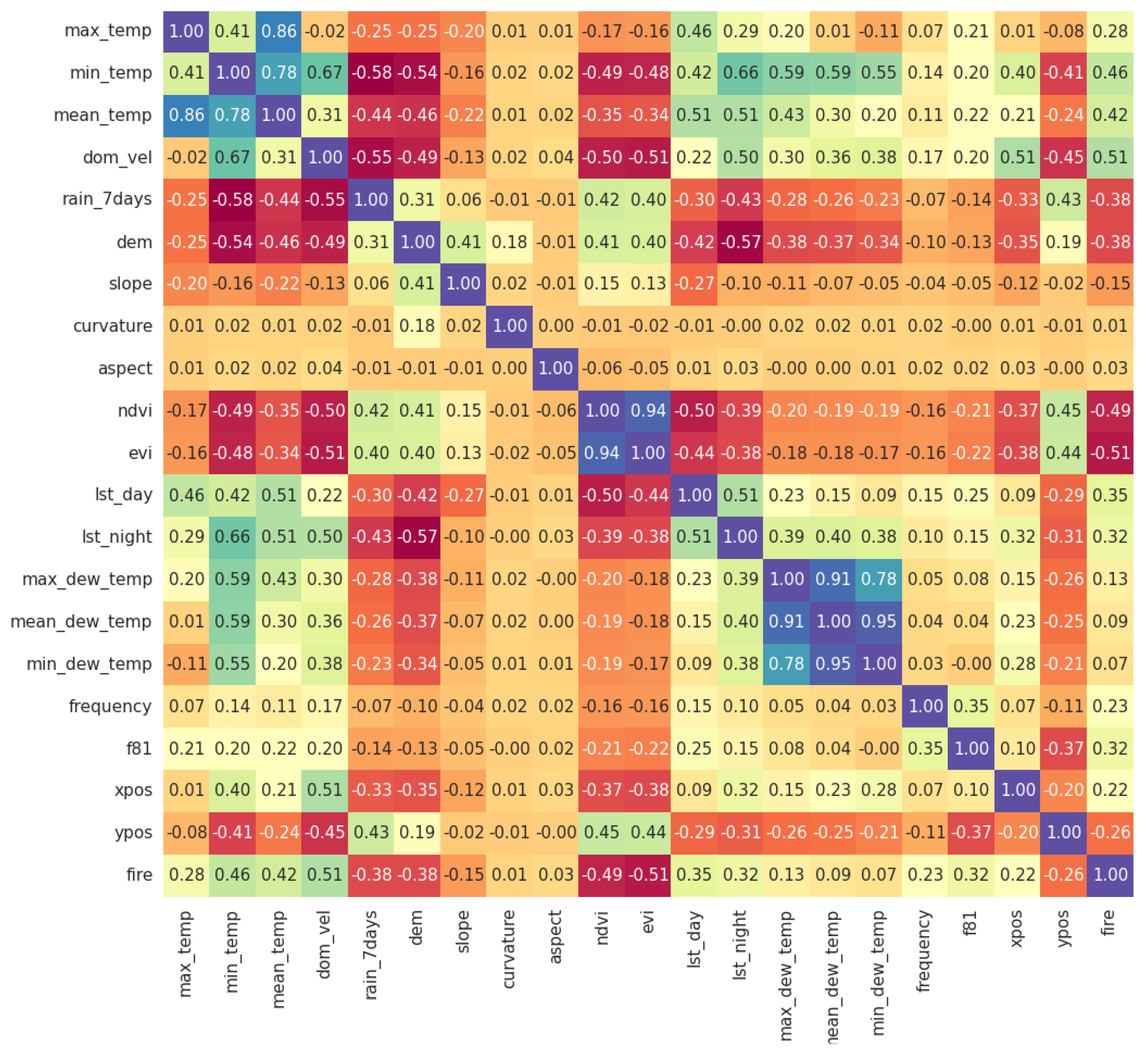
The above findings are further strengthened by examining the correlation between the features and the response variable. Figure 1 presents the values of Spearman’s correlation for all available numerical features. We can observe that almost all introduced features (except for dewpoint temperature ones) present absolute correlation values of more that , reaching up to .
We note that the above schemes (permutation importance and feature correlation) can only serve as indication and not as proof of the (the degree of) importance of the examined features. For example, permutation importance can be problematic when there are strong correlations between training features. On the other hand, Spearman’s correlation is able to capture only monotonic correlations between variables, while the ML algorithms we deploy are able to identify and exploit more complex (e.g., non-monotonic) relations. Nevertheless, the findings on feature importance provided by the two above schemes, in conjunction with the comparative findings of Section 4.2.1, provide strong indications about the utility of the newly introduced training features.
4.2.3. Gains from Hybrid Measures and Alternative Cross Validation Scheme
In Table 5 we present the effectiveness (sensitivity/specificity) scores achieved by the proposed models on the 2019 test set. In this table, we analyze the contribution of the task specific, hybrid evaluation measures for model selection, as well as the alternative cross-validation scheme, that were presented in Section 3.2. The tested models were chosen from both cross validation schemes for each measure as described in Section 4.1. We emphasize here that the top row of the table refers to the measures that were used during cross-validation to select the best model, which is then assessed in terms of sensitivity/specificity (second row of the table) on the test set.
The first observation is that the proposed hybrid measures perform much better than the traditional ones (AUC and f-score). Given the empirical and practical requirement of achieving sensitivity close to and specificity , the best models we can obtain from the two traditional measures achieve values of , , (RF-AUC-defCV, RF-fscore-defCV, NN-AUC-altCV respectively), with the latter being achieved via the proposed alternative cross-validation scheme. On the other hand, the hybrid measures provide a variety of models with better performance, indicatively marked with bold in Table 5. For example, all models based on sh5 measure and the default cross-validation consistently achieve at least sensitivity with specificity ranging from to , while NNd-sh2-defCV achieves values of , which can be considered the best performance according to the aforementioned empirical requirement.
Additionally, in general, we can observe a slightly better performance of NN models compared to the tree ensemble algorithms and in particular regarding the NN with drop-out. This can be potentially/partly justified by the fact that some hurtful features were removed from NNs early on on the experimental process, since they were empirically shown to severely hurt their performance (Section 3.1), while they were left as is for the tree ensembles, since they seemed more robust at handling them at the time. Nevertheless, a more in-depth analysis of this effect is part of our ongoing work.
Another observation regards the expected trade-off between sensitivity and specificity scores for each model, as higher values of the first lead to lower values of the second and vice versa. Given this, we can see that the proposed hybrid measures can be used to increasingly adjust this trade-off in favor of sensitivity; moving rightward in each row of the table, most of the times sensitivity increases while specificity decreases. This is a useful behavior that allows the configurable selection of different models, when the needs on effectiveness slightly differ.
Comparing the performance of the two cross-validation schemes, we observe that when focusing on models with very high sensitivity, the default scheme performs slightly better than the alternative one, with the differences being in the order of 1–3% in most cases, e.g., when examining the best models from both schemes in the sh5 measure column. One possible explanation is the fact that, as described in Section 3.2.2, not being able to use as validation set the whole respective dataset, but only of it, we are still missing significant information from the initial data distribution. The information gain compared to the default scheme (which maintains a marginal percentage from the initial dataset for validation) seems to not be adequate to compensate for the decreased number of hyperparameterizations that are searched. On the other hand, considering scenarios where sensitivity can drop to 80–85% in favor of increased specificity, we can observe that the alternative cross-validation scheme and, in particular, combined with rh2 measure, provides the most suitable/balanced models via RF and ET ((, ( respectively). This indicates some tangible gains on specificity, i.e., that the alternative scheme does capture some additional, useful information regarding the no-fire instances of the initial data distribution. Our ongoing work investigates more optimal schemes for balancing the aforementioned trade-off.
4.2.4. Model Generalization
To obtain an indication of how well our proposed models generalize through different years (without re-training), we handpick several models with good performance on the 2019 test set and present them in Table 6. There, we compare their performance between the 2019 and the 2020 test set. The results in the 2020 test set demonstrate an increased performance w.r.t. sensitivity, reaching nearly optimal values of 95% to 98%, compared to the 2019 test set, where the values range from 90% to 94%. A somehow higher volatility though for the sensitivity measure is expected if we account for the huge imbalance between the classes (Section 4.1 and Section 5.1, Table 2). On the other hand, the specificity values demonstrate a relative stability, as the metric difference per model between the two test sets is in the range 0–2% (e.g., RF-sh5-defCV, ET-rh5-altCV, NN-rh5-defCV, NNd-sh2-defCV, NN-auc-altCV) with the exception of a few models of which the difference is in the range 3–4% (e.g., NN-sh5-altCV, NNd-sh5-altCV, NNd-sh10-altCV). The above findings indicate that our models can generalize well in terms of both measures, allowing the selection of models that achieve values of at least in both test years.
5. Discussion
Next day fire prediction comprises an open and quite challenging problem, which is reflected by the fact that, in its realistic formulation that we consider in this work, it is hardly handled in the existing literature [8,14,43]. On the contrary, most works (see Section 1) focus on related but quite different problem formulations, regarding the problem setting and challenges, such as next week/month/year fire prediction or fire susceptibility prediction. As a result, the majority of such works do not handle real-world characteristics of the next day fire prediction problem, such as extreme scale and imbalance, proposing methods that cannot be operationally adopted by fire services in real-world scenarios. In the current work, we introduce a ML methodology and models that can effectively solve the task, achieving sensitivity and specificity values at the levels of and on a yearly level, on real-world test sets covering a whole country. Such values render our proposed models already more effective than existing operational systems, such as the one published from the Greek Civil Protection Agency that operates on prefecture level (https://www.civilprotection.gr/el/daily-fire-prediction-map; accessed on 22 February 2022). Further, the proposed methodology adheres to strict best practices that rule out the possibility of data leakage and ensure the generalizability of the fire prediction models. Nevertheless, through our analysis we identify room for improvement in several aspects of the task, as analyzed next.
5.1. Data Scale and Imbalance
To handle the massive amounts of extremely imbalanced training data, we resort to the widely adopted solution of undersampling the majority class (no-fire) instances. However, no matter how sophisticated the undersampling process might be, it is expected to severely change the distribution of the data, since only a marginal percentage of the initial no-fire instances is left in the dataset (in case we aim for a balanced training set). In particular, the initial fire to no-fire instances ratio is 1:100 K and drops to 1:1, meaning that only of the initial no-fire instances are kept in the final, balanced training set. This means that a large amount of potentially very informative no-fire instances, with respect to differentiating against fire instances, are inevitably removed from the training set. Thus, any ML model that is utilized, however effective it might be, is trained on a different distribution than the one that is finally tested/deployed on. On the other hand, maintaining the initial distribution is practically computationally inefficient as analyzed in Section 3.2.1. In this work, we tried to partially ameliorate the above significant issue, by assessing the trained models on validation sets that are much closer (size-wise) to the initial data sizes (alternative cross-validation scheme in Section 3.2.2), aiming this way to maintain as much of the initial data distribution as possible. Although some positive indications on the value of such a process were identified (see Section 4.2.3), in general it did not clearly improve the effectiveness of the model and needs further investigation and potential enhancements planned in our future work.
Further, we recognize that the above scheme is practically a “half-measure”, or at least one side of the coin, for the discussed problem. This is because it only targets at a more proper selection (on validation sets) of models (algorithm hyperparameterizations) that are trained on a changed distribution, thus already inherit a bias from this training. Namely, even if a cross-validation scheme is very effective in selecting the proper models with respect to the real-world data distribution, it is still limited in selecting from a pool of models that are trained on a different (undersampled) distribution. Therefore, more sophisticated schemes need to be devised for the construction of more informative and close to the real-world distribution training sets. Uniformly undersampling both classes in order to maintain the exact initial ratio is out of the question due to the extreme class imbalance that leads to absolute rarity [39]. e.g., reducing the 830 M dataset by a factor of 100 is expected to lead to just over 100 fire instances, depriving the training set of valuable information. This gets even worse if we take into account the rigidness of most existing algorithmic frameworks in training models on imbalance data [39]. On the other hand, a set of initial, ongoing experiments we are currently conducting indicate that simply performing a more limited undersampling process on the majority class (e.g., dropping from 1:100 K to 1:1000 fire to no-fire instances) might not be adequate and most probably needs to be combined with more targeted/task-specific sampling process for the no-fire class. This needs to take into account properties of the data, such as rare cases [39] or absence of fire. Rare cases are identified when a certain class (fire class in our case) is comprised of several individual “cases”, i.e., groups of instances that might considerably differ to each other, but are classified to the same class—for example, areas with different topological characteristics that had a fire occurrence.
Absence of fire on the other hand comprises an opposite issue: no-fire areas that had very similar characteristics with fire areas. It has to be emphasized that those labels do not declare true absence of fire, because it is not known with absolute certainty whether a fire could not occur (and thus to be a true absence), or simply did not happen for “random” reasons [12]. In reality those labels are used as pseudo-absence data because the task we handle needs to be formalized as a binary classification problem. In general, the feature representations of no-fire instances can be very similar to the ones of fire instances (hard instances [44]), or very different (easy instances) that make extremely unlike a fire to occur, or lie between these two extremes (semi-hard instances). A training set that contains too many no-fire instances similar to fire ones (hard instances) could potentially make the training process extremely difficult, resulting either to a model that predicts many fire instances as no-fire or to a very complex-overfitted model that has struggled to learn to discriminate between the two classes essentially based on noise. On the other hand, if a training set contains too many no-fire instances very different to fire ones (easy instances) it will make the training process easier but it will produce models that struggle to decide (and thus perform poorly, potentially achieving very low specificity values) when an area’s conditions are not extreme in favor of either classes.
A statistical analysis of the features and (intra- and inter-class) similarities between the instances of fire and no-fire classes and between the instances of each class itself would be helpful towards obtaining a better understanding of the training set and, at a further step, for optimizing the sampling the no-fire instances. Especially given the fact that, for different scenarios, sampling of different types of instances might be more appropriate [44,45]. In our setting, several sampling strategies could be compared or combined, in order to obtain a training set as close to the initial dataset distribution as possible. Re-assigning “absence of fire” areas from no-fire to fire class is one option, as performed in [6], where the authors consider buffers around fire cells and denote no-fire cells lying within the buffers as fire ones. Of course this oversampling process needs to be performed exclusively on the training set, and not be extended to the test set as done in the specific work. Another option would be to further investigate rare cases within the fire class instances and potentially handle them as separate classes, facilitating thus the classifier into better discriminating these cases into more canonical spaces within the feature hyperspace. Further, improving the majority class undersampling process from random selection towards the obligatory consideration of semi-hard no-fire instances as a percentage of the eventually sampled set could potentially assist the learning process; the optimization algorithm would this way focus on discriminating inter-class instances that are meaningfully distant to each other and would potentially produce more robust models.
5.2. Concept Drifts and Model Robustness
Wildfires are highly volatile phenomena, often affected by factors that are quite difficult to be captured and encoded as training features, such as arson, accidentally human-induced fires, lightning, power pole sparkles, etc. The training features that we are able to utilize essentially describe the proneness of an area regarding fire occurrence. Further, there exist temporal correlations, also difficult to capture, through consecutive years. For example, having an excess of fire occurrences during a year might lead to high operational alertness during the next year, which can potentially dramatically reduce fire occurrences (more than what would otherwise be expected). The best chance at handling this problem lies at devising features that could, even implicitly or partially, encode such information. Example of such features are the fire history and spatially smoothed fire history, which are already proposed in this work and seem to contribute (Section 4.2.2) to the improvement of the ML prediction algorithms. Additional features that could be examined regard the general “context” of an area, such as the proximity to urban or agricultural territories, the density of existing buildings/structures, the surrounding road network [46], etc. Further, it is probably worth examining socio-economic and demographic (e.g., population density) features, since they have been widely used in various earth observation modelling and analysis tasks [47].
Apart from the above, dataset shift [48] is an inherent problem in the specific task. Take for example meteorological conditions that can highly vary through the months of the same year, as well as gradually change through the course of years due to climate change. The effects of the former (variability in data distribution through different months) can be implicitly observed in Table 3, where the effectiveness values for the same models are lower for month August compared to the average yearly effectiveness (especially regarding specificity), meaning that for some of the other months the models are much more effective. These heterogeneous behaviors indicate that implementing individual models for different months of each year could potentially help better dealing with this heterogeneity. Going a step further, experimenting with ensemble schemes that learn to differently weight these individual models might be a promising direction towards ameliorating the above heterogeneity and dataset shifts.
5.3. Deep Learning
Deep learning (DL) has recently overwhelmed the research community, presenting great advancements in machine vision (e.g., image classification, object detection) and sequential tasks (e.g., natural language processing). The most common paradigm of DL methods is neural network architectures with many hidden layers, accompanied, depending on the task, by several specific schemes (e.g., recurrent gates, convolutions, normalization layers, dropout layers, encoder/decoder/attention mechanisms, etc.) [36]. Nevertheless, it is often the case that ML problems comprising tabular data (such as in our case) tree ensemble algorithms present superior performance [49,50], depending though on the task and the underlying data.
In our work up until now, we have extensively studied tree ensembles and shallow NNs on the task, having also in mind the important hardware restrictions of the task in a real-world deployment scenario. However, we do believe that DL methods have a high potential for further improving the currently reported prediction effectiveness. In particular, we have identified two directions to be explored in our future work.
Siamese Neural Networks and Outlier Detection. Casting the fire prediction task as an outlier detection problem, with supervised deep metric learning approaches such as Siamese networks [51] and Triplet networks for extremity recognition comprises a first direction. These types of architectures tend to bring semantically similar samples closer and dissimilar samples further away in the latent representation space. In our research, we plan to exploit this behavior combined with optimized cost functions, in order to learn new spaces of distributed representations (embeddings) and identify out-of-distribution samples (i.e., areas that are likely to be on fire) [52]. In previous works, it has been stated that metric learning performs well in tasks with high imbalance [53], while, to the best of our knowledge this type of methods has not yet been assessed on EO data and fire risk prediction in particular.
Convolutional Neural Networks and Bayesian CNN. In this study, we explored the tabular aspect of the instances at hand, i.e., for each area we extracted numerical vectors as representations. However, another viewpoint of the problem can consider the area-grid cells as a 2-dimensional plane/image. In such a setting, Convolutional Neural Networks (CNN) [54] can be deployed, like in [6], so that the inherent spatial correlations of the data can be better captured/utilized. In our future work, we particularly plan to assess semantic segmentation algorithms, i.e., CNNs that exploit labeling information in the level of pixel (cell), such as Fully Convolutional Networks, U-nets, etc. [55]. Furthermore, and in order to incorporate a measure of the certainty in the class selection probability which implies the fire risk, we will attempt to exploit Bayesian CNN algorithms that combine CNNs with the ability of Bayesian methods to measure the certainty of the algorithm’s decision [56].
Finally, overall, the aforementioned DNN-oriented research directions will facilitate the exploitation of larger parts of the available data for training/validation.
5.4. Operational Mode
The presented work is not limited to a “laboratory” setting; on the contrary it is implemented into an integrated pre-operational environment that has been producing daily maps during the wildfire season of 2021 for the whole Greek territory. This environment, which is shared with the Greek Fire Service, facilitates the continuous assessment and evaluation of the proposed methods on a daily basis, as well as the gradual embracement of the proposed technologies by the Fire Service. Each cell in the produced maps is assigned a level of risk (in a five-grade scale) using the probability of fire to no-fire class selection by the model’s prediction.
An indicative risk map of 4 August 2021 is presented in Figure 2 (left map), where the fire events of that day are indicated by a location marker. The zoomed rectangles around the map correspond to all the ignition points. We can observe that all the fire events of that day were located in cells predicted with high risk of fire (>0.8 probability of “fire” class selection) by our system. The map on the right in Figure 2 is the published fire risk map of the same day by the Civil Protection Agency where the risk is provided at prefecture level. Although the Civil Protection risk map may be used for various purposes, like public awareness, it is evident that the fine-grained resolution of our predictions, compared to the highly coarse one of the Civil Protection, is of much higher utility for operational organization of the Fire Service. In particular, for the specific day, the Civil Protection map has annotated the whole Greek territory as medium and high risk; on the other hand, our map identifies very high risk areas, while it also assigns a considerable proportion of areas to low and no risk.
Furthermore, apart from the continuous assessment, the proposed solution is continuously enhanced considering various components.For example, the meteorology features are currently in the process of being enhanced to higher resolution provided by the operational NOA/BEYOND numerical weather prediction method, which is an implementation of WRF-ARW atmospheric model [57], and runs daily in NOA/BEYOND premises. This will result to obtaining meteorology features of a higher-resolution (2 km grid spacing as compared to the currently used, coarser granularity of 9 km) over Greece. That allows for a significantly more detailed representation of the meteorology driving factors for wildfire compared to the ERA5-land dataset.
6. Conclusions
In this paper we presented a ML methodology and models for handling the problem of next day wildfire prediction in the scale of a country. The proposed methods aim at solving (some of) the several lacks and shortcomings in existing works of the literature, while based on the analysis of a large wildfire dataset we have created, and the results we achieve, we discuss directions for future exploration. Further, our proposed methods achieve adequately high effectiveness scores (sensitivity > 90%, specificity > 65%) and are realized within a pre-operational environment that is continuously assessed on real-world conditions and also improved based on the feedback of the Greek Fire Service.
Author Contributions
Conceptualization C.K.; formal analysis, A.A., S.G. and G.G.; data curation, A.A., S.G. and N.S.B.; writing—original draft preparation, G.G., A.A., S.G. and N.S.B.; writing—review and editing, A.A., G.G. and S.G.; visualization, A.A. and S.G.; funding acquisition, C.K. All authors have read and agreed to the published version of the manuscript.
Funding
This paper has been supported by using data and resources from the following Project funded the Greek Government—Ministry of Development & Investments: CLIMPACT: Flagship Initiative for Climate Change and its Impact by the Hellenic Network of Agencies for Climate Impact Mitigation and Adaptation.
Data Availability Statement
The data presented in this study are available on request from the corresponding author. The data are not publicly available due to particular infrastructure requirements that need to be satisfied, including appropriate data sharing approvals that need to be obtained first from individual sources where data were obtained from.
Conflicts of Interest
The authors declare no conflict of interest.
Appendix A. Hyperparameter Spaces
In this Appendix we subjoin the hyperparameter spaces as they were structured in python code for the hyperopt library. Function hp.quniform(label, low, high, q) returns a value like . Function hp.choice(label, options) returns one of the options in a list or a tuple. The elements of options can themselves be nested stochastic expressions.
Appendix A.1. FCNN Parameter Space
space_FCNN = {’n_internal_layers’: hp.choice(’n_internal_layers’,
[
(0, {’layer_1_0_nodes’: hp.quniform(’layer_1_0_w_nodes’, 100, 2100, 100)}),
(1, {’layer_1_1_nodes’: hp.quniform(’layer_1_1_w_nodes’, 100, 2100, 100),
’layer_2_1_nodes’: hp.quniform(’layer_2_1_w_nodes’, 100, 2100, 100)}),
(2, {’layer_1_2_nodes’: hp.quniform(’layer_1_2_w_nodes’, 100, 2100, 100),
’layer_2_2_nodes’: hp.quniform(’layer_2_2_w_nodes’, 100, 2100, 100),
’layer_3_2_nodes’: hp.quniform(’layer_3_2_w_nodes’, 100, 2100, 100)}),
(3, {’layer_1_3_nodes’: hp.quniform(’layer_1_3_w_nodes’, 100, 2100, 100),
’layer_2_3_nodes’: hp.quniform(’layer_2_3_w_nodes’, 100, 2100, 100),
’layer_3_3_nodes’: hp.quniform(’layer_3_3_w_nodes’, 100, 2100, 100),
’layer_4_3_nodes’: hp.quniform(’layer_4_3_w_nodes’, 100, 2100, 100)}),
(0, {’layer_1_0_nodes’: hp.quniform(’layer_1_0_nodes’, 10, 100, 10)}),
(1, {’layer_1_1_nodes’: hp.quniform(’layer_1_1_nodes’, 10, 100, 10),
’layer_2_1_nodes’: hp.quniform(’layer_2_1_nodes’, 10, 100, 10)}),
(2, {’layer_1_2_nodes’: hp.quniform(’layer_1_2_nodes’, 10, 100, 10),
’layer_2_2_nodes’: hp.quniform(’layer_2_2_nodes’, 10, 100, 10),
’layer_3_2_nodes’: hp.quniform(’layer_3_2_nodes’, 10, 100, 10)}),
(3, {’layer_1_3_nodes’: hp.quniform(’layer_1_3_nodes’, 10, 100, 10),
’layer_2_3_nodes’: hp.quniform(’layer_2_3_nodes’, 10, 100, 10),
’layer_3_3_nodes’: hp.quniform(’layer_3_3_nodes’, 10, 100, 10),
’layer_4_3_nodes’: hp.quniform(’layer_4_3_nodes’, 10, 100, 10)}),
(4, {’layer_1_4_nodes’: hp.quniform(’layer_1_4_nodes’, 10, 100, 10),
’layer_2_4_nodes’: hp.quniform(’layer_2_4_nodes’, 10, 100, 10),
’layer_3_4_nodes’: hp.quniform(’layer_3_4_nodes’, 10, 100, 10),
’layer_4_4_nodes’: hp.quniform(’layer_4_4_nodes’, 10, 100, 10),
’layer_5_4_nodes’: hp.quniform(’layer_5_4_nodes’, 10, 100, 10)})
]
),
’dropout’: hp.choice(’dropout’,[0.1, 0.2, 0.3]),
#’dropout’: hp.choice(’dropout’,[None]),
’class_weights’: hp.choice(’class_weights’, [{0:1, 1:1}, {0:1, 1:2}, {0:2,1:3},
{0:1, 1:5}, {0:1, 1:10}]),
’feature_drop’: hp.choice(’feature_drop’,[[’dir_max’, ’dom_dir’,’month’, ’wkd’]]),
’max_epochs’: hp.choice(’max_epochs’, [2000]),
’optimizer’: hp.choice(’optimizer’,[
{’name’:’Adam’,’adam_params’:hp.choice(’adam_params’,[None])}]),
’ES_monitor’:hp.choice(’ES_monitor’, [’loss’]),
’ES_patience’:hp.choice(’ES_patience’, [10]),
’ES_mindelta’:hp.choice(’ES_mindelta’, [0.0001]),
’batch_size’:hp.choice(’batch_size’, [512])
}
Appendix A.2. Ensemble Trees Algorithms Parameter Spaces
space_RF = {’algo’: hp.choice(’algo’, [’RF’]),
’n_estimators’: hp.choice(’n_estimators’, [50, 100, 120, 150,170,200, 250, 350,
500, 750, 1000,1400, 1500]),
’min_samples_split’: hp.choice(’min_samples_split’,[2, 10, 50, 70,100,120,150,180,
200, 250,400,600,1000, 1300, 2000]),
’min_samples_leaf’ :hp.choice(’min_samples_leaf’,[1, 10,30,40,50,100,120,150]),
’criterion’:hp.choice(’criterion’,["gini", "entropy"]),
’max_features’:hp.quniform(’max_features’, 1,10,1), # the x/10 of the total features
’bootstrap’:hp.choice(’bootstrap’,[True, False]),
’max_depth’: hp.choice(’max_depth’, [10, 20, 100, 200, 400,500, 700, 1000, 1200,2000, None]),
’feature_drop’: hp.choice(’feature_drop’, [[]]),
’class_weights’:hp.choice(’class_weight’,[{0:1,1:300},{0:1,1:400},{0:1,1:500},{0:1,1:1000}])
}
space_XT = { ’algo’: hp.choice(’algo’, [’XT’]),
’n_estimators’: hp.choice(’n_estimators’,[10, 20, 40, 60, 80, 100, 200, 400, 600, 800, 1000]),
’criterion’: hp.choice(’criterion’,[’gini’, ’entropy’]),
’max_depth’: hp.quniform(’max_depth’,2, 40, 2),
’min_samples_split’: hp.choice(’min_samples_split’,[2, 10, 50, 70, 100, 120, 150, 180,
200, 250, 400, 600, 1000, 1300, 2000]),
’min_samples_leaf’: hp.choice(’min_samples_leaf’,[5, 10, 15, 20, 25, 30, 35, 40, 45]),
’max_features’: hp.quniform(’max_features’, 1,10,1), # the x/10 of the total features
’bootstrap’: hp.choice(’bootstrap’,[True, False]),
’class_weights’: hp.choice(’class_weights’,[{0: 4, 1: 6}, {0: 1, 1: 10}, {0: 1, 1: 50},
{0: 1, 1: 70}]),
’feature_drop’: [],
}
space_XGB = { ’algo’: hp.choice(’algo’, [’XGB’]),
’max_depth’: hp.quniform(’max_depth’,2, 100, 2),
’n_estimators’: hp.choice(’n_estimators’,[10, 20, 40, 60, 80, 100, 200, 400, 600, 800, 1000]),
’subsample’: hp.choice(’subsample’,[0.5, 0.6, 0.7, 0.8, 0.9, 1]),
’alpha’: hp.choice(’alpha’, [0, 1, 10, 20, 40, 60, 80, 100]),
’gamma’: hp.choice(’gamma’,[0, 0.001, 0.01, 0.1, 1, 10, 100, 1000]),
’lambda’: hp.quniform(’lambda’,1, 22, 1),
’scale_pos_weight’: hp.choice(’scale_pos_weight’,[9, 15, 50, 70, 100, 200, 500]),
’feature_drop’: [],
}
References
- Jain, P.; Coogan, S.C.; Subramanian, S.G.; Crowley, M.; Taylor, S.; Flannigan, M.D. A review of machine learning applications in wildfire science and management. Environ. Rev. 2020, 28, 478–505. [Google Scholar] [CrossRef]
- Tonini, M.; D’Andrea, M.; Biondi, G.; Degli Esposti, S.; Trucchia, A.; Fiorucci, P. A Machine Learning-Based Approach for Wildfire Susceptibility Mapping. The Case Study of the Liguria Region in Italy. Geosciences 2020, 10, 105. [Google Scholar] [CrossRef] [Green Version]
- Gigović, L.; Pourghasemi, H.R.; Drobnjak, S.; Bai, S. Testing a New Ensemble Model Based on SVM and Random Forest in Forest Fire Susceptibility Assessment and Its Mapping in Serbia’s Tara National Park. Forests 2019, 10, 408. [Google Scholar] [CrossRef] [Green Version]
- Rodrigues, M.; de la Riva, J. An insight into machine-learning algorithms to model human-caused wildfire occurrence. Environ. Model. Softw. 2014, 57, 192–201. [Google Scholar] [CrossRef]
- Tehrany, M.; Jones, S.; Shabani, F.; Martínez-Álvarez, F.; Bui, D. A Novel Ensemble Modelling Approach for the Spatial Prediction of Tropical Forest Fire Susceptibility Using Logitboost Machine Learning Classifier and Multi-source Geospatial Data. Theor. Appl. Climatol. 2019, 137, 637–653. [Google Scholar] [CrossRef]
- Zhang, G.; Wang, M.; Liu, K. Forest Fire Susceptibility Modeling Using a Convolutional Neural Network for Yunnan Province of China. Int. J. Disaster Risk Sci. 2019, 10, 386–403. [Google Scholar] [CrossRef] [Green Version]
- Wu, Z.; Li, M.; Wang, B.; Quan, Y.; Liu, J. Using Artificial Intelligence to Estimate the Probability of Forest Fires in Heilongjiang, Northeast China. Remote Sens. 2021, 13, 1813. [Google Scholar] [CrossRef]
- Alonso-Betanzos, A.; Fontenla-Romero, O.; Guijarro-Berdiñas, B.; Hernández-Pereira, E.; Inmaculada Paz Andrade, M.; Jiménez, E.; Luis Legido Soto, J.; Carballas, T. An intelligent system for forest fire risk prediction and fire fighting management in Galicia. Expert Syst. Appl. 2003, 25, 545–554. [Google Scholar] [CrossRef]
- Vasilakos, C.; Kalabokidis, K.; Hatzopoulos, J.; Kallos, G.; Matsinos, Y. Integrating new methods and tools in fire danger rating. Int. J. Wildland Fire 2007, 16, 306–316. [Google Scholar] [CrossRef]
- Stojanova, D.; Kobler, A.; Ogrinc, P.; Ženko, B.; Džeroski, S. Estimating the risk of fire outbreaks in the natural environment. Data Min. Knowl. Discov. 2012, 24, 411–442. [Google Scholar] [CrossRef]
- Bisquert, M.; Caselles, E.; Sánchez, J.M.; Caselles, V. Application of artificial neural networks and logistic regression to the prediction of forest fire danger in Galicia using MODIS data. Int. J. Wildland Fire 2012, 21, 1025–1029. [Google Scholar] [CrossRef]
- Massada, A.B.; Syphard, A.; Stewart, S.I.; Radeloff, V. Wildfire ignition-distribution modelling: A comparative study in the Huron-Manistee National Forest, Michigan, USA. Int. J. Wildland Fire 2013, 22, 174–183. [Google Scholar] [CrossRef]
- Apostolakis, A.; Girtsou, S.; Kontoes, C.; Papoutsis, I.; Tsoutsos, M. Implementation of a Random Forest Classifier to Examine Wildfire Predictive Modelling in Greece Using Diachronically Collected Fire Occurrence and Fire Mapping Data. In Proceedings of the MultiMedia Modeling—27th International Conference, MMM 2021, Prague, Czech Republic, 22–24 June2021; Lokoc, J., Skopal, T., Schoeffmann, K., Mezaris, V., Li, X., Vrochidis, S., Patras, I., Eds.; Springer: Berlin/Heidelberg, Germany, 2021; Volume 12573, pp. 318–329. [Google Scholar] [CrossRef]
- Girtsou, S.; Apostolakis, A.; Giannopoulos, G.; Kontoes, C. A Machine Learning methodology for next day wildfire prediction. In Proceedings of the 2021 IEEE International Geoscience and Remote Sensing Symposium IGARSS, Brussels, Belgium, 11–16 July 2021. [Google Scholar]
- Yerushalmy, J. Statistical Problems in Assessing Methods of Medical Diagnosis, with Special Reference to X-ray Techniques. Public Health Rep. (1896–1970) 1947, 62, 1432–1449. [Google Scholar] [CrossRef]
- Kontoes, C.; Keramitsoglou, I.; Papoutsis, I.; Sifakis, N.; Xofis, P. National Scale Operational Mapping of Burnt Areas as a Tool for the Better Understanding of Contemporary Wildfire Patterns and Regimes. Sensors 2013, 13, 11146–11166. [Google Scholar] [CrossRef] [Green Version]
- Hellenic National Meteorological Service.Climate Atlas of Greece. Available online: http://climatlas.hnms.gr/sdi/?lang=EN (accessed on 22 February 2022).
- © European Union. Copernicus Land Monitoring Service 2018; European Environment Agency (EEA). Available online: https://land.copernicus.eu/pan-european/corine-land-cover/clc2018 (accessed on 22 February 2022).
- Pausas, J. Changes in fire and climate in the Eastern Iberian Peninsula (Mediterranean Basin). Clim. Chang. 2004, 63, 337–350. [Google Scholar] [CrossRef]
- Pausas, J.; Fernández-Muñoz, S. Fire regime changes in the Western Mediterranean Basin: From fuel-limited to drought-driven fire regime. Clim. Chang. 2012, 110, 215–226. [Google Scholar] [CrossRef] [Green Version]
- Lancaster, D. A Review of Some Image Pixel Interpolation Algorithms. 2012. Available online: https://www.tinaja.com/glib/pixintpl.pdf (accessed on 22 February 2022).
- Hancock, J.T.; Khoshgoftaar, T.M.; Hancock, K.J. Survey on categorical data for neural networks. Big Data 2020, 7, 28. [Google Scholar] [CrossRef] [Green Version]
- Zumbrunnen, T.; Pezzatti, G.B.; Menéndez, P.; Bugmann, H.; Bürgi, M.; Conedera, M. Weather and human impacts on forest fires: 100 years of fire history in two climatic regions of Switzerland. For. Ecol. Manag. 2011, 261, 2188–2199. [Google Scholar] [CrossRef]
- Ganteaume, A.; Camia, A.; Jappiot, M.; San-Miguel-Ayanz, J.; Long-Fournel, M.; Lampin, C. A review of the main driving factors of forest fire ignition over Europe. Environ. Manag. 2013, 51, 651–662. [Google Scholar] [CrossRef] [Green Version]
- Maselli, F.; Romanelli, S.; Bottai, L.; Zipoli, G. Use of NOAA-AVHRR NDVI images for the estimation of dynamic fire risk in Mediterranean areas. Remote Sens. Environ. 2003, 86, 187–197. [Google Scholar] [CrossRef]
- Huete, A.; Didan, K.; Miura, T.; Rodriguez, E.; Gao, X.; Ferreira, L. Overview of the radiometric and biophysical performance of the MODIS vegetation indices. Remote Sens. Environ. 2002, 83, 195–213. [Google Scholar] [CrossRef]
- Matsushita, B.; Yang, W.; Chen, J.; Yuyichi, O.; Guoyu, Q. Sensitivity of the Enhanced Vegetation Index (EVI) and Normalized Difference Vegetation Index (NDVI) to Topographic Effects: A Case Study in High-Density Cypress Forest. Sensors 2007, 7, 2636. [Google Scholar] [CrossRef] [PubMed] [Green Version]
- Maffei, C.; Alfieri, S.; Menenti, M. Time Series of Land Surface Temperature from Daily MODIS Measurements for the Prediction of Fire Hazard; 2014; pp. 1024–1029. Available online: https://www.researchgate.net/profile/Carmine-Maffei/publication/271646072_Time_series_of_land_surface_temperature_from_daily_MODIS_measurements_for_the_prediction_of_fire_hazard/links/54cea28a0cf298d65661e2a9/Time-series-of-land-surface-temperature-from-daily-MODIS-measurements-for-the-prediction-of-fire-hazard.pdf (accessed on 22 February 2022).
- Pulfer, E.M. Different Approaches to Blurring Digital Images and Their Effect on Facial Detection. Bachelor Thesis, University of Arkansas, Fayetteville, AR, USA, 2019. [Google Scholar]
- Forsyth, D.A.; Ponce, J. Computer Vision—A Modern Approach, 2nd ed.; Prentice Hall: Hoboken, NJ, USA, 2012; pp. 1–791. [Google Scholar]
- Vasilakos, C.; Kostas, A.E.; Ae, K.; Hatzopoulos, J.; Vasilakos, C.; Hatzopoulos, J.; Matsinos, Á.I.; Kalabokidis, K. Identifying Wildland Fire Ignition Factors through Sensitivity Analysis of a Neural Network. Nat. Hazards 2009, 50, 125–143. [Google Scholar] [CrossRef]
- Breiman, L. Random Forests. Mach. Learn. 2001, 45, 5–32. [Google Scholar] [CrossRef] [Green Version]
- Geurts, P.; Ernst, D.; Wehenkel, L. Extremely randomized trees. Mach. Learn. 2006, 63, 3–42. [Google Scholar] [CrossRef] [Green Version]
- Chen, T.; Guestrin, C. XGBoost. In Proceedings of the 22nd ACM SIGKDD International Conference on Knowledge Discovery and Data Mining, San Francisco, CA, USA, 13–17 August 2016. [Google Scholar] [CrossRef] [Green Version]
- McCulloch, W.S.; Pitts, W. A logical calculus of the ideas immanent in nervous activity. Bull. Math. Biophys. 1943, 5, 115–133. [Google Scholar] [CrossRef]
- Goodfellow, I.; Bengio, Y.; Courville, A. Deep Learning; MIT Press: Cambridge, MA, USA, 2016; Available online: http://www.deeplearningbook.org (accessed on 22 February 2022).
- Kingma, D.P.; Ba, J. Adam: A Method for Stochastic Optimization. arXiv 2017, arXiv:1412.6980. [Google Scholar]
- Srivastava, N.; Hinton, G.; Krizhevsky, A.; Sutskever, I.; Salakhutdinov, R. Dropout: A Simple Way to Prevent Neural Networks from Overfitting. J. Mach. Learn. Res. 2014, 15, 1929–1958. [Google Scholar]
- He, H.; Ma, Y. Imbalanced Learning: Foundations, Algorithms, and Applications, 1st ed.; Wiley-IEEE Press: Hoboken, NJ, USA, 2013. [Google Scholar]
- Rijsbergen, C.J.V. Information Retrieval, 2nd ed.; Butterworth-Heinemann: Oxford, UK, 1979. [Google Scholar]
- Youden, W.J. Index for rating diagnostic tests. Cancer 1950, 3, 32–35. [Google Scholar] [CrossRef]
- Fawcett, T. An introduction to ROC analysis. Pattern Recognit. Lett. 2006, 27, 861–874. [Google Scholar] [CrossRef]
- Padilla, M.; Vega-Garcia, C. On the comparative importance of fire danger rating indices and their integration with spatial and temporal variables for predicting daily human-caused fire occurrence in Span. Int. J. Wildland Fire 2011, 20, 46–58. [Google Scholar] [CrossRef]
- Schroff, F.; Kalenichenko, D.; Philbin, J. FaceNet: A Unified Embedding for Face Recognition and Clustering. In Proceedings of the IEEE Conference on Computer Vision and Pattern Recognition (CVPR), Boston, MA, USA, 7–12 June 2015; pp. 815–823. [Google Scholar] [CrossRef] [Green Version]
- Yuan, Y.; Chen, W.; Yang, Y.; Wang, Z. In Defense of the Triplet Loss Again: Learning Robust Person Re-Identification with Fast Approximated Triplet Loss and Label Distillation. In Proceedings of the IEEE/CVF Conference on Computer Vision and Pattern Recognition (CVPR) Workshops, Seattle, WA, USA, 14–19 June 2020; pp. 1454–1463. [Google Scholar] [CrossRef]
- Mitsakis, E.; Stamos, I.; Papanikolaou, A.; Ayfantopoulou, G.; Charalabos, K. Assessment of extreme weather events on transport networks: Case study of the 2007 wildfires in Peloponnesus. Nat. Hazards 2014, 72, 87–107. [Google Scholar] [CrossRef]
- Parselia, E.; Charalabos, K.; Tsouni, A.; Hadjichristodoulou, C.; Kioutsioukis, I.; Magiorkinis, G.; Stilianakis, N. Satellite Earth Observation Data in Epidemiological Modeling of Malaria, Dengue and West Nile Virus: A Scoping Review. Remote Sens. 2019, 11, 1862. [Google Scholar] [CrossRef] [Green Version]
- Quionero-Candela, J.; Sugiyama, M.; Schwaighofer, A.; Lawrence, N. Dataset Shift in Machine Learning; MIT Press: Cambridge, MA, USA, 2009. [Google Scholar]
- Klambauer, G.; Unterthiner, T.; Mayr, A.; Hochreiter, S. Self-Normalizing Neural Networks. In Proceedings of the 31st International Conference on Neural Information Processing Systems, Long Beach, CA, USA, 4–9 December 2017; Curran Associates Inc.: Red Hook, NY, USA, 2017; pp. 972–981. [Google Scholar]
- Gorishniy, Y.; Rubachev, I.; Khrulkov, V.; Babenko, A. Revisiting Deep Learning Models for Tabular Data. arXiv 2021, arXiv:2106.11959. [Google Scholar]
- Vijay Kumar, B.; Carneiro, G.; Reid, I. Learning Local Image Descriptors with Deep Siamese and Triplet Convolutional Networks by Minimizing Global Loss Functions. In Proceedings of the 2016 IEEE Conference on Computer Vision and Pattern Recognition (CVPR), Las Vegas, NV, USA, 27–30 June 2016; pp. 5385–5394. [Google Scholar] [CrossRef]
- Yu, L.; Twardowski, B.; Liu, X.; Herranz, L.; Wang, K.; Cheng, Y.; Jui, S.; van de Weijer, J. Semantic Drift Compensation for Class-Incremental Learning. In Proceedings of the 2020 IEEE/CVF Conference on Computer Vision and Pattern Recognition (CVPR), Seattle, WA, USA, 13–19 June 2020. [Google Scholar]
- Drozdov, I.; Szubert, B.; Cole, J.; Monaco, C. Structure-preserving visualisation of high dimensional single-cell datasets. Sci. Rep. 2019, 9, 8914. [Google Scholar]
- Bengio, Y.; Lecun, Y. Convolutional Networks for Images, Speech, and Time-Series. Handb. Brain Theory Neural Netw. 1997, 3361, 1995. [Google Scholar]
- Minaee, S.; Boykov, Y.; Porikli, F.; Plaza, A.; Kehtarnavaz, N.; Terzopoulos, D. Image Segmentation Using Deep Learning: A Survey. IEEE Trans. Pattern Anal. Mach. Intell. 2020. [Google Scholar] [CrossRef]
- Gal, Y.; Ghahramani, Z. Bayesian Convolutional Neural Networks with Bernoulli Approximate Variational Inference. arXiv 2016, arXiv:1506.02158. [Google Scholar]
- Skamarock, C.; Klemp, B.; Dudhia, J.; Gill, O.; Liu, Z.; Berner, J.; Wang, W.; Powers, G.; Duda, G.; Barker, D.; et al. A Description of the Advanced Research WRF Model Version 4; National Center for Atmospheric Research: Boulder, CO, USA, 2019. [Google Scholar]
Figure 1.
Spearman’s correlation values between problem’s independent (training features) and dependent (fire occurrence to be predicted) variables.
Figure 1.
Spearman’s correlation values between problem’s independent (training features) and dependent (fire occurrence to be predicted) variables.

Figure 2.
Daily wildfire risk map. The map on the left is created by our pre-operational system for 4 August 2021; the provided resolution is 500 m. The map on the right is the official daily map published by civil protection agency for the same day; the resolution is on prefecture level.
Figure 2.
Daily wildfire risk map. The map on the left is created by our pre-operational system for 4 August 2021; the provided resolution is 500 m. The map on the right is the official daily map published by civil protection agency for the same day; the resolution is on prefecture level.

Table 2.
Distribution of fire and no-fire instances in the dataset.
| Year | August | Sum June–September | ||
|---|---|---|---|---|
| No Fire | Fire | No Fire | Fire | |
| 2010 | 11,687,055 | 347 | 45,995,051 | 607 |
| 2011 | 11,685,953 | 1468 | 45,993,489 | 2202 |
| 2012 | 11,685,532 | 1816 | 45,992,810 | 2806 |
| 2013 | 11,686,833 | 599 | 45,994,470 | 1233 |
| 2014 | 11,687,130 | 304 | 45,994,809 | 899 |
| 2015 | 11,687,290 | 144 | 45,994,915 | 793 |
| 2016 | 11,687,188 | 246 | 45,993,758 | 1950 |
| 2017 | 11,686,508 | 926 | 45,994,210 | 1498 |
| 2018 | 11,687,345 | 87 | 45,995,092 | 598 |
| 2019 | 11,562,808 | 386 | 45,100,739 | 631 |
| 2020 | 11,560,400 | 221 | 44,926,467 | 749 |
Table 3.
Effectiveness (sensitivity/specificity) of the proposed models, compared to [14] on the 2019 test set. In the first column the model is referenced as “Algorithm-Cross Validation measure-Cross Validation scheme” (see Section 4.1) and in the parentheses next to the model we denote the origin of the results (current work or IGARSS 2021 [14]). The second column contains the sensitivity and specificity scores for August 2019 test set while the third column contains the same measures averaged on the most significant months of the wildfire period: June, July, August, and September.
| # | Algorithm/Model | August 2019 | June–September 2019 | ||
|---|---|---|---|---|---|
| Sens. | Spec. | Sens. | Spec. | ||
| 1 | NN-AUC-defCV (igarss21) | 0.87 | 0.42 | - | - |
| 2 | RF-AUC-defCV (igarss21) | 0.92 | 0.36 | - | - |
| 3 | XG-rh5-defCV (igarss21) | 0.91 | 0.39 | - | - |
| 4 | NN-rh5-defCV (current) | 0.90 | 0.51 | 0.90 | 0.66 |
| 5 | NNd-sh5-altCV (current) | 0.94 | 0.47 | 0.90 | 0.62 |
| 6 | RF-sh5-defCV (current) | 0.89 | 0.42 | 0.90 | 0.55 |
| 7 | XG-sh5-defCV (current) | 0.91 | 0.46 | 0.91 | 0.56 |
| 8 | ET-sh5-defCV (current) | 0.92 | 0.38 | 0.94 | 0.54 |
| 9 | ET-rh5-altCV (current) | 0.91 | 0.47 | 0.92 | 0.59 |
Table 4.
Feature ranking using permutation importance with three of the best models emerged from tests for algorithms NNd (FCNN with dropout layer), RF and XGB.
Table 4.
Feature ranking using permutation importance with three of the best models emerged from tests for algorithms NNd (FCNN with dropout layer), RF and XGB.
| Rank | NNd (nh2-defCV) | RF (nh5-defCV) | XGB (nh5-defCV) | |||
|---|---|---|---|---|---|---|
| Feature | Imp. (%) | Feature | Imp. (%) | Feature | Imp. (%) | |
| 1 | dom_vel | 6.07 | dom_vel | 12.94 | dom_vel | 7.47 |
| 2 | evi | 2.38 | evi | 2.37 | evi | 2.24 |
| 3 | f81 | 1.99 | f81 | 2.18 | dem | 1.68 |
| 4 | xpos | 1.47 | ndvi_new | 2.13 | max_temp | 1.63 |
| 5 | xpos | 1.18 | mean_temp | 1.72 | xpos | 1.58 |
| 6 | dem | 1.17 | max_temp | 1.71 | xpos | 1.48 |
| 7 | rain_7days | 0.57 | lst_day | 1.48 | f81 | 1.36 |
| 8 | max_temp | 0.44 | xpos | 1.20 | rain_7days | 0.80 |
| 9 | frequency | 0.26 | xpos | 1.12 | mean_dew_temp | 0.67 |
| 10 | slope | 0.19 | mean_dew_temp | 1.11 | mean_temp | 0.47 |
Table 5.
Comparative scores of the different measures from both the default and the alternative cross validation scheme on test set 2019.
Table 5.
Comparative scores of the different measures from both the default and the alternative cross validation scheme on test set 2019.
| Algo | AUC | f-Score | rh2 | rh5 | sh2 | sh5 | sh10 | |||||||
|---|---|---|---|---|---|---|---|---|---|---|---|---|---|---|
| Sens. | Spec. | Sens. | Spec. | Sens. | Spec. | Sens. | Spec. | Sens. | Spec. | Sens. | Spec. | Sens. | Spec. | |
| Default (k-fold) Cross-Validation | ||||||||||||||
| RF | 0.87 | 0.66 | 0.86 | 0.67 | 0.78 | 0.71 | 0.88 | 0.59 | 0.87 | 0.61 | 0.90 | 0.55 | 0.94 | 0.47 |
| ET | 0.57 | 0.83 | 0.79 | 0.69 | 0.75 | 0.73 | 0.81 | 0.68 | 0.79 | 0.69 | 0.94 | 0.54 | 0.79 | 0.68 |
| XGB | 0.54 | 0.80 | 0.57 | 0.75 | 0.67 | 0.74 | 0.74 | 0.69 | 0.68 | 0.71 | 0.91 | 0.56 | 0.93 | 0.51 |
| NN | 0.71 | 0.77 | 0.67 | 0.80 | 0.72 | 0.78 | 0.90 | 0.66 | 0.83 | 0.68 | 0.92 | 0.58 | 0.96 | 0.47 |
| NNd | 0.66 | 0.84 | 0.77 | 0.78 | 0.79 | 0.76 | 0.91 | 0.65 | 0.90 | 0.67 | 0.93 | 0.59 | 0.97 | 0.47 |
| Alternative Cross-Validation | ||||||||||||||
| RF | 0.74 | 0.80 | 0.13 | 0.99 | 0.82 | 0.71 | 0.87 | 0.64 | 0.91 | 0.47 | 0.91 | 0.47 | 0.91 | 0.47 |
| ET | 0.32 | 0.96 | 0.27 | 0.97 | 0.85 | 0.69 | 0.92 | 0.59 | 0.94 | 0.52 | 0.93 | 0.52 | 0.95 | 0.45 |
| XGB | 0.70 | 0.77 | 0.34 | 0.94 | 0.74 | 0.69 | 0.82 | 0.62 | 0.91 | 0.59 | 0.95 | 0.46 | 0.95 | 0.46 |
| NN | 0.90 | 0.61 | 0.48 | 0.88 | 0.84 | 0.67 | 0.90 | 0.61 | 0.84 | 0.64 | 0.91 | 0.61 | 0.93 | 0.62 |
| NNd | 0.81 | 0.71 | 0.51 | 0.87 | 0.85 | 0.68 | 0.89 | 0.64 | 0.88 | 0.66 | 0.91 | 0.59 | 0.91 | 0.61 |
Table 6.
Comparison of average yearly results on 2019 and 2020 test sets.
| Model | 2019 | 2020 | ||
|---|---|---|---|---|
| Sens. | Spec. | Sens. | Spec. | |
| RF-sh5-defCV | 0.90 | 0.55 | 0.97 | 0.56 |
| ET-sh5-defCV | 0.94 | 0.54 | 0.97 | 0.54 |
| XGB-sh5-defCV | 0.91 | 0.56 | 0.97 | 0.58 |
| XGB-sh10-defCV | 0.93 | 0.51 | 0.98 | 0.52 |
| ET-rh5-altCV | 0.92 | 0.59 | 0.96 | 0.59 |
| ET-sh2-altCV | 0.94 | 0.52 | 0.98 | 0.52 |
| ET-sh5-altCV | 0.93 | 0.52 | 0.98 | 0.52 |
| XGB-sh2-altCV | 0.91 | 0.59 | 0.96 | 0.58 |
| NN-rh5-defCV | 0.90 | 0.66 | 0.95 | 0.67 |
| NNd-rh5-defCV | 0.91 | 0.65 | 0.95 | 0.66 |
| NNd-sh2-defCV | 0.90 | 0.67 | 0.95 | 0.67 |
| NN-sh5-defCV | 0.92 | 0.58 | 0.95 | 0.59 |
| NNd-sh5-defCV | 0.93 | 0.59 | 0.96 | 0.62 |
| NN-auc-altCV | 0.90 | 0.61 | 0.97 | 0.59 |
| NN-rh5-altCV | 0.90 | 0.61 | 0.97 | 0.58 |
| NN-sh5-altCV | 0.91 | 0.61 | 0.96 | 0.58 |
| NNd-sh5-altCV | 0.91 | 0.59 | 0.98 | 0.55 |
| NN-sh10-altCV | 0.93 | 0.62 | 0.97 | 0.58 |
| NNd-sh10-altCV | 0.91 | 0.61 | 0.97 | 0.60 |
Publisher’s Note: MDPI stays neutral with regard to jurisdictional claims in published maps and institutional affiliations. |
© 2022 by the authors. Licensee MDPI, Basel, Switzerland. This article is an open access article distributed under the terms and conditions of the Creative Commons Attribution (CC BY) license (https://creativecommons.org/licenses/by/4.0/).
Share and Cite
MDPI and ACS Style
Apostolakis, A.; Girtsou, S.; Giannopoulos, G.; Bartsotas, N.S.; Kontoes, C. Estimating Next Day’s Forest Fire Risk via a Complete Machine Learning Methodology. Remote Sens. 2022, 14, 1222. https://doi.org/10.3390/rs14051222
AMA Style
Apostolakis A, Girtsou S, Giannopoulos G, Bartsotas NS, Kontoes C. Estimating Next Day’s Forest Fire Risk via a Complete Machine Learning Methodology. Remote Sensing. 2022; 14(5):1222. https://doi.org/10.3390/rs14051222
Chicago/Turabian StyleApostolakis, Alexis, Stella Girtsou, Giorgos Giannopoulos, Nikolaos S. Bartsotas, and Charalampos Kontoes. 2022. "Estimating Next Day’s Forest Fire Risk via a Complete Machine Learning Methodology" Remote Sensing 14, no. 5: 1222. https://doi.org/10.3390/rs14051222
Note that from the first issue of 2016, this journal uses article numbers instead of page numbers. See further details here.