Calculator Notes for TI-89, TI-92 Plus, and Voyage 200

CHAPTER 13 Calculator Notes for the TI-89, TI-92 Plus, 

and Voyage 200 

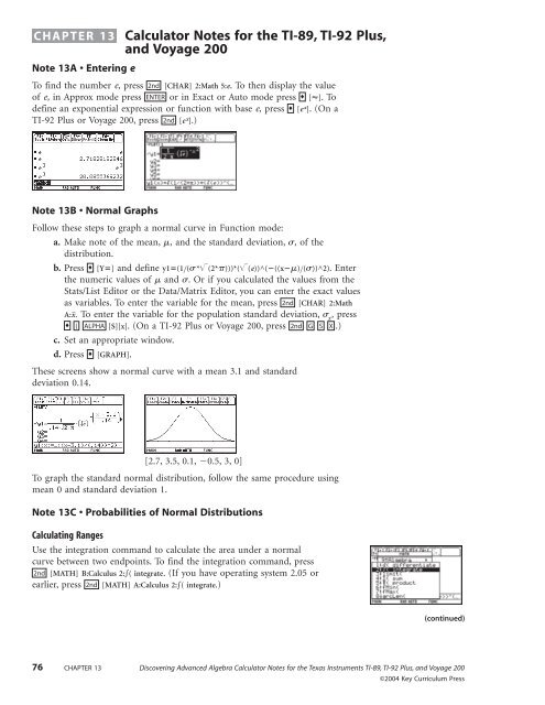
Note 13A • Entering e 

To find the number e, press [CHAR] 2:Math 5:e. To then display the value 

of e, in Approx mode press or in Exact or Auto mode press []. To 

define an exponential expression or function with base e, press [e x ]. (On a 

TI-92 Plus or Voyage 200, press [e x 2nd 

ENTER 

♦ 

♦ 

2nd ].) 

Note 13B • Normal Graphs 

Follow these steps to graph a normal curve in Function mode: 

a. Make note of the mean, , and the standard deviation, , of the 

distribution. 

b. Press ♦ [Y] and define y1(1( *(2*)))*((e))^(((x)())^2). Enter 

the numeric values of and . Or if you calculated the values from the 

Stats/List Editor or the Data/Matrix Editor, you can enter the exact values 

as variables. To enter the variable for the mean, press 2nd [CHAR] 2:Math 

A:x. To enter the variable for the population standard deviation, x , press 

♦ ( ALPHA [S][x]. (On a TI-92 Plus or Voyage 200, press 2nd G S X .) 

c. Set an appropriate window. 

d. Press ♦ [GRAPH]. 

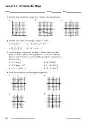
These screens show a normal curve with a mean 3.1 and standard 

deviation 0.14. 

[2.7, 3.5, 0.1, 0.5, 3, 0] 

To graph the standard normal distribution, follow the same procedure using 

mean 0 and standard deviation 1. 

Note 13C • Probabilities of Normal Distributions 

Calculating Ranges 

Use the integration command to calculate the area under a normal 

curve between two endpoints. To find the integration command, press 

[MATH] B:Calculus 2:( integrate. (If you have operating system 2.05 or 

2nd 

earlier, press 2nd [MATH] A:Calculus 2:( integrate.) 

(continued) 

76 CHAPTER 13 Discovering Advanced Algebra Calculator Notes for the Texas Instruments TI-89, TI-92 Plus, and Voyage 200 

©2004 Key Curriculum Press

Note 13C • Probabilities of Normal Distributions (continued) TI-89/TI-92 Plus/Voyage 200 

Before using the command, first enter the equation of the normal curve into 

the Y Editor screen. (See Note 13B.) Then on the Home screen, enter the 

integration command in the form ∫(y1(x),x,lower, upper). 

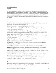
Graphing Ranges 

The calculator does not have a command that automatically draws a normal 

curve and shades the area under it. The best you can do is calculate the area, 

as explained above, and then graph a system of inequalities that shows the 

area as a feasible region. (Review Note 6G for help with graphing 

inequalities.) 

Your system should include these four equations: 

y1 the equation of your normal curve. Shade above y1. 

y2 0. Shade below y2. 

y3 1000(lowerx). Shade below y3. 

y4 1000(upperx). Shade above y4. 

[2.7, 3.5, 0.1, 0.5, 3, 0] 

Probabilities of Normal Distributions with the Stats/List Editor 

If your calculator has the Stats/List Editor application, you can use built-in 

functions that calculate and graph the area under a normal curve. To run the 

Stats/List Editor, press APPS 1:FlashApps and select Stats/List Editor. 

The normal cumulative distribution function, Normal Cdf, calculates the 

area between two endpoints. You find the Normal Cdf command by pressing 

F5 (Distr) 4:Normal Cdf. Enter the Lower Value, the Upper Value, the mean, and the 

standard deviation, and then press ENTER . 

Discovering Advanced Algebra Calculator Notes for the Texas Instruments TI-89, TI-92 Plus, and Voyage 200 CHAPTER 13 77 

©2004 Key Curriculum Press 

(continued)

Note 13C • Probabilities of Normal Distributions (continued) TI-89/TI-92 Plus/Voyage 200 

The Shade Normal command graphs and calculates the area between two 

endpoints. You find this command by pressing F5 (Distr) 1:Shade 1:Shade 

Normal. Enter the Lower Value, the Upper Value, the mean, and the standard 

deviation, set Auto-scale to YES, and then press ENTER . (Note: Auto-scale adjusts 

the window to fit the normal curve. If you have already set an appropriate 

window, you can choose NO.) 

Note 13D • Creating Random Probability Distributions 

You can create lists of various kinds of distributions. To create each list, you 

must press 2nd [MATH] 3:List 1:seq(. 

a. To create a uniform distribution, use 2nd [MATH] 7:Probability 4:rand(. 

In this example, the command seq(2030rand(),x,1,200)→p1 creates a list 

of 200 values uniformly distributed between 20 and 50. 

[20, 50, 2, 0, 50, 1] 

b. To create a normal distribution, use 2nd [MATH] 7:Probability 5:randNorm(. 

In this example, the command seq(randNorm(35,5),x,1,200)→p1 creates a list 

of 200 values with mean 35 and standard deviation 5. Almost all of the 

values will be between 20 and 50. 

[20, 50, 2, 0, 50, 1] 

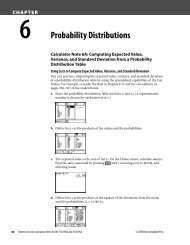
c. To create a left-skewed distribution, use the cube root of rand(. In this 

example, the command seq(2030(rand())^(13),x,1,200)→p1 creates a 

left-skewed population of 200 values between 20 and 50. 

[20, 50, 2, 0, 50, 1] 

(continued) 



Note 13D • Creating Random Probability Distributions (continued) TI-89/TI-92 Plus/Voyage 200 

d. To create a right-skewed distribution, use the cube of rand(. In this 

example, the command seq(2030(rand())^3,x,1,200)→p1 creates a 

right-skewed population of 200 values between 20 and 50. 

[20, 50, 2, 0, 50, 1] 

Note 13E • Sampling from a Distribution 

Before starting the sampling routine, make sure that you have stored your 

distribution into a list p1 (see Note 13D), calculated the population mean 

and standard deviation, and graphed y1, y22x and y32x. 

Now, the recursive routine below will randomly choose one value at a time 

from list p1 and add it to a sample, and then plot a point in the form 

(number sampled, sample mean). In the routine, the variable n is the number 

sampled and the variable t is the sum of the data values. Hence, the routine 

plots the point (n, tn). 

a. Initialize n to 0 by pressing 0 STOÍ alpha [N] ENTER . 

b. Initialize t to 0 by pressing 0 STOÍ T ENTER . 

c. Enter this recursive routine on the Home screen: 

n1→n: tp1[rand(200)]→t: PtOn n, tn 

Find the rand( command by pressing 2nd [MATH] 7:Probability 4:rand(. Find 

the point plotting command, PtOn, by pressing CATALOG [P] and scrolling 

down to PtOn. Get the colon by pressing 2nd [:]. 

d. Begin the sampling-and-plotting routine by pressing ENTER HOME ENTER 

HOME , and so on. Each time you press ENTER , you’ll see a new point 

plotted on the graph. 

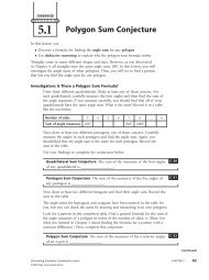
Note 13F • Correlation Coefficient 

[0, 50, 10, 20, 20, 1] 

There are two ways to find a correlation coefficient, r, using your calculator. 

You can manually enter the calculations yourself, or you can have the 

calculator do the work for you. 

First store your bivariate data into two lists, say list w1 for the x-values and 

list w2 for the y-values. 



(continued)

Note 13F • Correlation Coefficient (continued) TI-89/TI-92 Plus/Voyage 200 

Follow these steps to manually calculate r: 

a. Calculate the two-variable statistics that you need for the formula by 

pressing 2nd [MATH] 6:Statistics 2:TwoVar ALPHA [W] 1 , ALPHA [W] 2 ENTER . 

The calculator calculates the statistics, but does not display them. You 

can display the statistics, if you like, by pressing 2nd 

8:ShowStat ENTER . 

[MATH] 6:Statistics 

(x x)(y y) 

b. Start inputting the formula on the Home screen by entering 

sxsy (n 1) 

sum((w1. Do not press ENTER yet. To find the sum( command, press 2nd 

[MATH] 3:List 6:sum(. 

c. Press 2nd [CHAR] 2:Math A:x to enter x into the expression. As an 

alternative, you can also enter mean(w1). Notice that by pressing 2nd 

[CHAR] 2:Math you can also get B:y. 

d. Enter the rest of the formula, ((w2y))(sx*sy*(nstat–1)). For sx and sy , 

simply type sx and sy. For n, type nstat. 

e. Press ENTER to display the value of r. 

Follow these steps to have the calculator compute r: 

a. From the Home screen, press 2nd [MATH] 6:Statistics 3:Regressions 1:LinReg 

alpha [W] 1 , alpha [W] 2 ENTER . 

Press 2nd [MATH] 6:Statistics 8:ShowStat ENTER to display the value of r, which 

is called corr. The calculator shows other information about the least 

squares line, which you’ll learn about later. 

You can also calculate r by choosing the LinReg command from the 

Data/Matrix Editor or the Stats/List Editor. Review Note 3D for finding a 

median-median line, but choose 5:LineReg for Calculation Type. 



Note 13G • LSL Program 

The program lsl allows you to adjust a line until the sum of the squares of 

the residuals is minimized. Follow these steps: 

a. Store your data into lists l1 and l2. 

b. Run the program. 

c. A short set of instructions are displayed. Arrow up or down to change the 

intercept of the line. Arrow left or right to change the slope of the line. 

Press CLEAR to reset the line and start over. Press ESC to quit the program. 

d. Press ENTER to see a scatter plot of your data, a line, and a physical 

representation of the squares of the residuals. (Note: The graphing 

window may not be square, so the squares may look like rectangles.) Keep 

adjusting the line until you have found the line with the smallest sum of 

the squared residuals, the value of sqr sum in the upper-left corner. 

Clean-Up 

After you quit the program, Plots 1, 2, and 3 remain on. Go to the 

Y Editor screen to clear them or turn them off so they do not interfere 

with future graphing activities. 

lsl() 

Prgm 

© Displays line of fit for data 

in l1, l2 and squares of 

residuals; allows adjustment 

© Instructions 

ClrIO 

Disp "Find line of fit" 

Disp "Up and dn:change intercept" 

Disp "Rt and left:change slope" 

Disp "CLEAR:reset ESC:quit" 

Disp "" 

Pause "To begin, press ENTER." 

PlotsOff 

FnOff 

setMode("Graph","FUNCTION") 

setMode("Angle","DEGREE") 

NewPlot 1,1,l1,l2,,,,3 © Plots 

data points 

ZoomData 

TI-89/TI-92 Plus/Voyage 200 



© Get stats for data 

dim(l1)ánum 

TwoVar l1,l2 

(num*∑xy-∑x*∑y)/(num*∑x2-∑x^2)áslope © Slope of least squares line 

© Store means in lists for 

plotting 

mean(l1)ámeanx:mean(l2)ámeany 

{meanx}ál3:{meany}ál 4 

NewPlot 2,1,l3,l4,,,,4 

© Copy vertical mean, slope for 

changing line 

slopeásl 

meanyáw 

© Set up lists for line of fit 

and residual squares 

seq(l1[int(x/5)+1],x,0,5*num-1)ál 5 

seq(l2[int(x/5)+1],x,0,5*num-1)ál 6 

(continued)

Note 13G • LSL Program (continued) TI-89/TI-92 Plus/Voyage 200 

(Program: lsl continued) 

© Extend lists with temporary 

values 

xmaxál5[5*num+1] 

ymaxál6[5*num+1] 

augment({xmin},l5)ál 5 

augment({ymin},l6)ál 6 

Loop 

© Fix l5, l6 for plotting 

For j,1,num 

l1[j]ádatax:l2[j]ádatay 

w+sl*(datax-meanx)áz 

zál6[5*j-3]:zál 6[5*j]:zál6[5*j+1] 

datax-(datay-z)áz 

zál5[5*j-1]:zál 5[5*j] 

EndFor 

© Adjust window to contain 

residual squares 

max(max(l5),xmax)áxmax 

min(min(l5),xmin)áxmin 

max(max(l6),ymax)áymax 

min(min(l6),ymin)áymin 

© Make first and last of l5 and 

l6 to draw line to edge of 

screen 

xminál 5[1] 

xmaxál5[5*num+2] 

w+sl*(xmin-meanx)ál 6[1] 

w+sl*(xmax-meanx)ál6[5*num+2] 

© Plot line of fit, with 

residual squares 

NewPlot 3,2,l5,l6,,,,5 

© Calculate residuals lr, sum r, 

sum of squares s, and plot 

l2-(w+sl*(l1-meanx))álr 

sum(lr)ár 

sum(lr^2)ás 

Note 13H • Least Squares Line 

(ymax-ymin)/102ác © Vertical 

shift amount 

PtText "res sum="&string 

(round(r,3)),xmin,ymax 

PtText "sqr sum="&string 

(round(s,3)),xmin,ymax-12*c 

© Show all plots 

DispG 

getKey()ák 

While k=0 

getKey()ák 

EndWhile 

If k=264 Then © ESC to quit 

Exit ©program 

ElseIf k=338 Then © up arrow; 

1 increment 

w+cáw 

ElseIf k=344 Then © down arrow; 

1 increment 

w-cáw 

ElseIf k=337 Then © left arrow; 

1 degree 

tan(tan -1 (sl)+1)ásl 

ElseIf k=340 Then © right arrow; 

1 degree 

tan(tan -1 (sl)-1)ásl 

ElseIf k=263 Then © CLEAR to 

reset 

EndIf 

slopeásl:meanyáw 

EndLoop 

DispHome 

EndPrgm 

The calculator can find the equation of the least squares line in the form 

y ax b. To use the command from the Home screen, press 2nd 

[MATH] 

6:Statistics 3:Regressions 1:LinReg followed by the names of the lists for the x- and 

y-values separated by a comma. Press ENTER to calculate the line. 

(continued) 



Note 13H • Least Squares Line (continued) TI-89/TI-92 Plus/Voyage 200 

To display the slope, y-intercept, correlation coefficient, and coefficient of 

determination, press 2nd [MATH] 6:Statistics 8:ShowStat ENTER . 

To enter the equation of the least squares line into the Y Editor, say in y1, 

type regeq(x)→y1(x) into the entry line on the Home screen, and press ENTER . 

You can also use the Data/Matrix Editor or the Stats/List Editor to calculate 

the least squares line. Follow the same procedure that you use to calculate a 

median-median line (see Note 3D), but choose 5:LinReg for Calculation Type. 

Note 13I • Nonlinear Regression 

The calculator uses a least squares approach to fit a curve to nonlinear data. 

It uses a combination of linearization and multivariable analysis. 

You can find all of these nonlinear regression commands in the 

6:Statistics 3:Regressions submenu: 

[MATH] 

2:ExpReg Exponential: y abx 3:QuadReg Quadratic: y ax2 bx c 

4:PwrReg Power: y axb 5:LnReg Logarithmic: y a b ln(x) 

7:CubicReg Cubic: y ax3 bx2 cx d 

8:QuartReg Quartic: y ax4 bx3 cx2 dx e 

9:SinReg Sinusoidal: y a sin(bx c) d 

A:Logistic Logistic: y c1 a ebx 2nd 

 

You enter each command followed by the names of the lists for the x- and 

y-values separated by a comma. 

The correlation coefficient, r, is not calculated for nonlinear regressions. 

However, quadratic, cubic, and quartic regressions give the coefficient of 

determination, R 2 .Some of the nonlinear regression commands have special 

requirements: 

Logarithmic regression must have all x-values greater than zero. 

Exponential and logistic regressions must have all y-values greater than zero. 

Power regression must have all x- and y-values greater than zero. 

Quadratic and logistic regressions require at least 3 points; cubic and sinusoidal 

regressions require at least 4 points; and quadratic regression requires at least 

5points. In general, a regression command needs at least as many points as 

there are parameters in the equation. 

You can also use the Data/Matrix Editor or the Stats/List Editor to calculate 

any of these regression models. Follow the same procedure that you use to 

calculate a median-median line (see Note 3D), but choose the appropriate 

regression model for Calculation Type.

Calculator Notes for TI-89, TI-92 Plus, and Voyage 200

You also want an ePaper? Increase the reach of your titles

Delete template?

Save as template?